R Graphics
[1]:
options.orig <- options(repr.plot.width=4, repr.plot.height=4)
Base Graphics
This is the graphics you get ont of the box, without loading any packages. It is not the prettiest, but great for quick plotting.
Scatter plot
[2]:
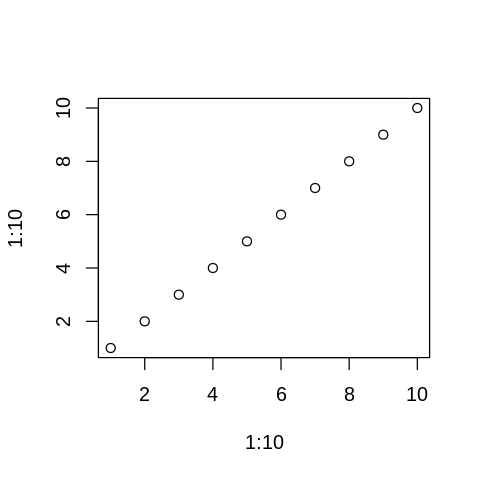
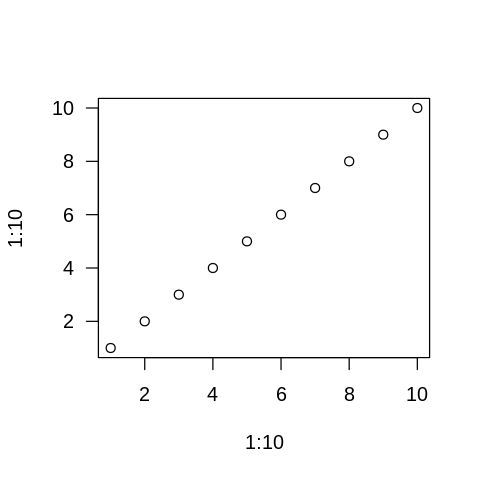
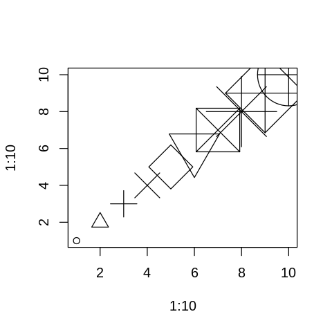
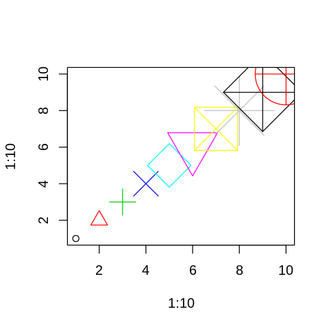
plot(1:10, 1:10)
Adding text labels
[7]:
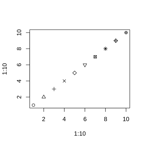
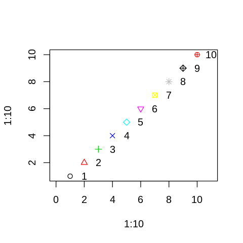
plot(1:10, 1:10, pch=1:10, col=1:10, xlim=c(0, 11))
text(1:10+1, 1:10, 1:10)
Line plot
[8]:
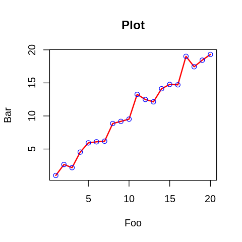
n <- 20
x <- 1:n
y <- x + rnorm(n)

plot(x, y, type="l", lty=1, lwd=2, col="red",
     main="Plot", xlab="Foo", ylab="Bar")
points(x, y, col="blue")
[9]:
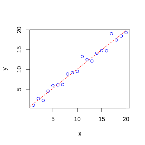
m <- lm(y ~ x)
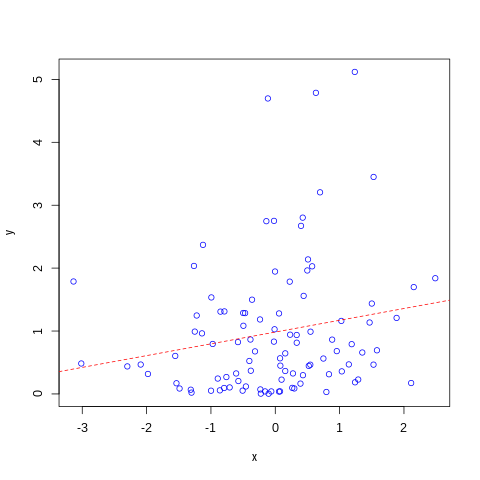
plot(x, y, col="blue")
abline(m, col="red", lty="dashed")
QQ plots
[14]:
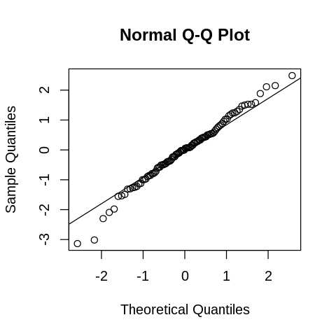
x <- rnorm(100)
[15]:
qqnorm(x)
qqline(x)
[16]:
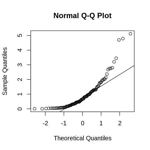
y <- rgamma(100, shape=1)
[17]:
qqnorm(y)
qqline(y)
Multiple plots
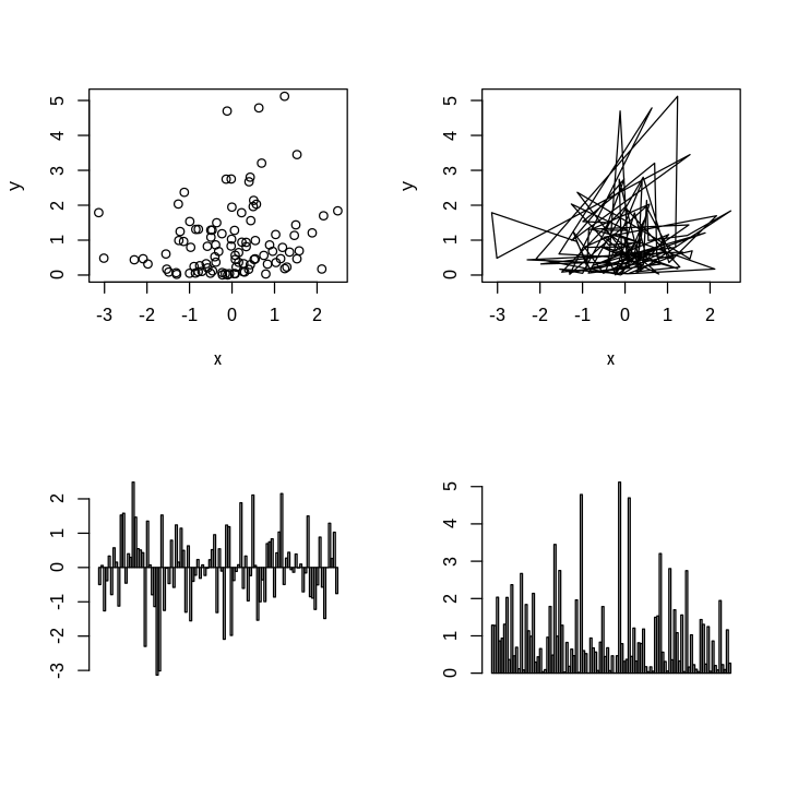
We can set up multiple plots with
par(mfrow=c(#rows, #cols))
where plots will be placed by row first
or
par(mfcol=c(#rows, #cols))
where plots will be placed by colum first.
[18]:
options.orig <- options(repr.plot.width=6, repr.plot.height=6)
[19]:
par(mfrow=c(2,2))
plot(x, y)
plot(x, y, type="l")
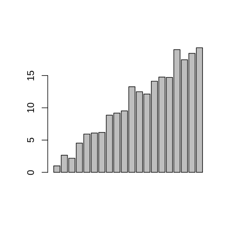
barplot(x)
barplot(y)
par(mfrow=c(1,1))
Saving plots
Saving a plot involves
opening a graphcis file device using
png(orpdf)issuing plot commands
then closing the device with
dev.off().
[20]:
png('figs/lm.png')
m <- lm(y ~ x)
plot(x, y, col="blue")
abline(m, col="red", lty="dashed")
dev.off()
png: 2
Retreive the PNG file