Simulations and Statistical Inference
[1]:
library(tidyverse)
Registered S3 methods overwritten by 'ggplot2':
  method         from
  [.quosures     rlang
  c.quosures     rlang
  print.quosures rlang
── Attaching packages ─────────────────────────────────────── tidyverse 1.2.1 ──
✔ ggplot2 3.1.1     ✔ purrr   0.3.2
✔ tibble  2.1.2     ✔ dplyr   0.8.1
✔ tidyr   0.8.3     ✔ stringr 1.4.0
✔ readr   1.3.1     ✔ forcats 0.4.0
── Conflicts ────────────────────────────────────────── tidyverse_conflicts() ──
✖ dplyr::filter() masks stats::filter()
✖ dplyr::lag()    masks stats::lag()
[2]:
options(repr.plot.width=4, repr.plot.height=3)
Set random number seed for reproducibility
[3]:
set.seed(42)
Generating numbers
Using the c function
[4]:
c(1,2,3,5,8,13)
- 1
- 2
- 3
- 5
- 8
- 13
Using the : operator
[5]:
1:10
- 1
- 2
- 3
- 4
- 5
- 6
- 7
- 8
- 9
- 10
[6]:
10:1
- 10
- 9
- 8
- 7
- 6
- 5
- 4
- 3
- 2
- 1
Using the seq function
[7]:
seq(1, 10)
- 1
- 2
- 3
- 4
- 5
- 6
- 7
- 8
- 9
- 10
[8]:
seq(1, 10, 2)
- 1
- 3
- 5
- 7
- 9
[9]:
seq(10, 1, -1)
- 10
- 9
- 8
- 7
- 6
- 5
- 4
- 3
- 2
- 1
[10]:
seq(0, 1, length.out = 11)
- 0
- 0.1
- 0.2
- 0.3
- 0.4
- 0.5
- 0.6
- 0.7
- 0.8
- 0.9
- 1
Using rep
rep is useful for generating repeating data patterns.
[11]:
rep(3, 5)
- 3
- 3
- 3
- 3
- 3
[12]:
rep(1:3, times=5)
- 1
- 2
- 3
- 1
- 2
- 3
- 1
- 2
- 3
- 1
- 2
- 3
- 1
- 2
- 3
[13]:
rep(1:3, each=5)
- 1
- 1
- 1
- 1
- 1
- 2
- 2
- 2
- 2
- 2
- 3
- 3
- 3
- 3
- 3
[14]:
rep(1:3, length.out=10)
- 1
- 2
- 3
- 1
- 2
- 3
- 1
- 2
- 3
- 1
Using sample
Simulate n tooses of a coin
[15]:
n <- 10
[16]:
t1 <- sample(c('H', 'T'), n, replace = TRUE)
t1
- 'H'
- 'H'
- 'H'
- 'H'
- 'T'
- 'T'
- 'T'
- 'T'
- 'H'
- 'T'
[17]:
table(t1)
t1
H T
5 5
Simulate n tosses of a biased coin
[18]:
t2 <- sample(c('H', 'T'), n, replace = TRUE, prob = c(0.3, 0.7))
t2
- 'T'
- 'H'
- 'H'
- 'T'
- 'T'
- 'H'
- 'H'
- 'T'
- 'T'
- 'T'
[19]:
table(t2)
t2
H T
4 6
Simulate n rolls of a 6-sided die
[20]:
n <- 100
[21]:
d1 <- sample(1:6, n, replace=TRUE)
d1
- 3
- 1
- 1
- 3
- 4
- 5
- 5
- 5
- 4
- 2
- 4
- 3
- 2
- 1
- 2
- 6
- 3
- 6
- 2
- 4
- 4
- 6
- 2
- 5
- 4
- 5
- 4
- 2
- 2
- 3
- 1
- 5
- 2
- 2
- 6
- 6
- 2
- 4
- 3
- 6
- 5
- 2
- 6
- 2
- 2
- 5
- 1
- 1
- 4
- 5
- 2
- 1
- 5
- 4
- 4
- 1
- 3
- 3
- 5
- 5
- 4
- 6
- 5
- 4
- 6
- 2
- 2
- 1
- 2
- 5
- 6
- 5
- 4
- 1
- 4
- 2
- 2
- 3
- 5
- 5
- 6
- 3
- 6
- 4
- 5
- 1
- 4
- 1
- 1
- 5
- 6
- 3
- 1
- 2
- 5
- 6
- 1
- 5
- 6
- 5
[22]:
table(d1)
d1
 1  2  3  4  5  6
15 20 11 17 22 15
Sampling without replacement. For example, if we wanted to assiggn 16 samples to treatment A or B at random such that exactly half had each treatment.
[23]:
sample(rep(c('A', 'B'), each=8))
- 'B'
- 'A'
- 'B'
- 'B'
- 'B'
- 'B'
- 'A'
- 'A'
- 'A'
- 'B'
- 'A'
- 'B'
- 'B'
- 'A'
- 'A'
- 'A'
Random number generators
Discrete distributions
Sampling from a Bernoullli distribution returns TRUE for success and FALSE for failure.
[24]:
rbernoulli(n=10, p=0.5)
- TRUE
- TRUE
- FALSE
- TRUE
- FALSE
- FALSE
- FALSE
- FALSE
- FALSE
- TRUE
[25]:
as.integer(rbernoulli(n=10, p=0.5))
- 0
- 0
- 0
- 0
- 0
- 1
- 1
- 1
- 1
- 1
Sampling from a Binomial distribution returns the number of successes in size trials for n experiments.
[26]:
rbinom(n=10, p=0.5, size=5)
- 4
- 2
- 2
- 3
- 3
- 4
- 3
- 1
- 2
- 2
Sampling from a negative binomial distribution returns the number of failures until size succcesses are observed for n experiemnts.
[27]:
rnbinom(n=10, size=5, prob=0.5)
- 4
- 0
- 9
- 4
- 2
- 4
- 6
- 5
- 5
- 4
Sampling from a Poisson distribution returns the number of successes in n experiments if the average success rate per experiment is lambda.
[28]:
rpois(n=10, lambda = 3)
- 5
- 2
- 1
- 0
- 2
- 2
- 1
- 2
- 0
- 9
Note: We can give different parameters for each experiment in these distributions.
[29]:
rpois(n=10, lambda=1:10)
- 2
- 0
- 5
- 4
- 4
- 3
- 7
- 4
- 7
- 10
Continuous distributions
Sampling from a standard uniform distribution.
[30]:
runif(5)
- 0.159469854552299
- 0.149578995071352
- 0.499272880377248
- 0.940564878052101
- 0.334231326589361
Sampling form a uniform distribution, with values between 90 and 100.
[31]:
runif(5, 90, 100)
- 91.8843432958238
- 92.6971617829986
- 95.3074407810345
- 90.2145022852346
- 97.987603074871
Sampling from a standard normal distribution.
[32]:
rnorm(5)
- -1.22474795035999
- 0.179516441117938
- 0.567620594423535
- -0.492877353553475
- 6.28840653511241e-05
Looping
[33]:
for (i in 1:10) {
    print(mean(rnorm(10)))
}
[1] 0.06091411
[1] -0.1028669
[1] -0.3117706
[1] 0.09639036
[1] 0.2010454
[1] -0.2384309
[1] 0.1271087
[1] -0.2115652
[1] -0.01946474
[1] -0.04661421
Saving variables generated in a loop
[34]:
n <- 10
vars <- numeric(n)
for (i in 1:n) {
    vars[i] <- mean(rnorm(10))
}
vars
- 0.102869685091412
- 0.0394963601049801
- 0.0587241371393688
- -0.208039597462606
- 0.175088960315561
- -0.0224984001571429
- 0.157365195356717
- -0.11380999366832
- -0.151701911199645
- 0.0806058319328881
[35]:
lapply(1:10,FUN = rnorm)
- 0.152764106747895
- 0.988596845178799
- -0.073458334672174
- -1.38702655355974
- -1.30667590437536
- -0.768395325077939
- -0.527108125374458
- -0.0214270650416246
- 0.670498070996282
- -0.434617038572407
- -1.11387978331285
- 0.6071059948785
- 0.275456968739591
- 1.15734706941474
- -1.68248085947826
- 0.0873190888948744
- 1.35336189394267
- 0.724173800683369
- -0.832552825764212
- 0.732528486768414
- -0.871926869997213
- -0.453397511229793
- 1.18753427862908
- -0.290145311790079
- 0.828546144965436
- -0.291227708779169
- -1.57636240474791
- -0.848815696948922
- -1.0885198619572
- -0.484290571117173
- -0.336311209009573
- -0.153357890661644
- -0.243247228574846
- 1.89220204160011
- -1.38599833728542
- -0.41482430070778
- 0.349081528106831
- 1.62844226581541
- 0.0885218957136163
- 1.23915070840056
- -1.64455553575371
- 1.44635652537848
- -0.690560171665183
- -0.276431085453852
- -1.10941875989944
- 0.133869316429452
- 1.78533905173155
- 2.42216335525159
- -1.07682890211841
- 0.485941110403099
- 1.38852173874429
- -0.195656817284544
- -0.218174797706211
- -0.304777954546445
- 0.597832724111443
[36]:
lapply(1:10, FUN = function(x) mean(rnorm(x)))
- 1.39742941081576
- 0.503903887768466
- -0.117686052712023
- 0.375071580419853
- 0.239310604458899
- 0.100315651769656
- -0.976662058729188
- -0.279974621278527
- 0.203381481503197
- 0.0364462992139071
Using replicate
replicate is like rep but works for a function (such as a random number generator)
[37]:
replicate(3, rnorm(5))
| -0.8673179 | -0.2785431 | -0.4034675 |
| 0.9506517 | 0.5461152 | 0.1046594 |
| -0.5850115 | -1.3038212 | -0.3188808 |
| 0.3209575 | -0.2509145 | 1.6183439 |
| -0.2993960 | 0.1710074 | 0.7141886 |
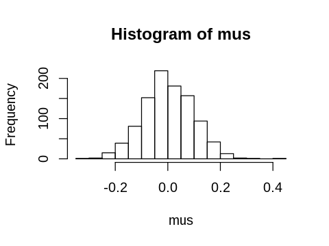
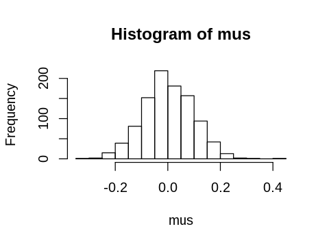
replicate is quite useful for simulations. For example, suppose we want to know the distribution of the sample mean if we sampled 100 numbers from the standard normal distribution 1,000 times.
[38]:
n_expts <- 1000
n <- 100
Using for loop
[39]:
set.seed(123)
mus <- numeric(n_expts)
for (i in 1:n_expts) {
    mus[i] <- mean(rnorm(n))
}
hist(mus)
Making a data.frame or tibble of simulated data
Let’s simulate the following experiment.
There are 10 subjects in Group A and 10 subjects in Group B with random PIDs from 10000-99999
We measure 5 genes in each subject. The genes have the same distribution for each subject, but different genes have different distribtutions:
gene1 \(\sim N(10, 1)\)
gene2 \(\sim N(11, 2)\)
gene3 \(\sim N(12, 3)\)
gene4 \(\sim N(13, 4)\)
gene5 \(\sim (N(14, 5)\)
NB: This is for illustration purposes! Our gene counts (even if ‘normalized’) are not normally distributed!
[41]:
replicate(5, rnorm(3, 1:5, 1))
| 1.264993 | 0.9467906 | 1.076689 | -1.503406 | 1.069951 |
| 3.830747 | 2.4379042 | 2.455073 | 1.404136 | 3.169101 |
| 2.940622 | 4.3374490 | 3.873871 | 2.264472 | 1.632268 |
[42]:
n <- 10
n_genes <- 5
min_pid <- 10000
max_pid <- 99999
groupings <- c('A', 'B')
n_groups <- length(groupings)
gene_mus <- 10:14
gene_sigmas <- 1:5
pad_width <- 3
[43]:
pids <- sample(min_pid:max_pid, n_groups*n)
groups <- sample(rep(groupings, each=n))
genes <- t(replicate(n_groups*n, rnorm(n_genes, gene_mus, gene_sigmas)))
gene_names <- paste('gene', str_pad(1:n_genes, width = pad_width, pad='0'), sep='')
colnames(genes) <- gene_names
[44]:
df <- tibble(
    pid = pids,
    grp = groups,
    genes
)
[45]:
sample_n(df, 3)
| pid | grp | genes |
|---|---|---|
| <int> | <chr> | <dbl[,5]> |
| 97320 | A | 9.532829, 11.047354, 14.08499, 14.35483, 22.422266 |
| 50148 | B | 10.046358, 11.926989, 14.43202, 14.20053, 14.613053 |
| 86850 | A | 9.535037, 9.418596, 13.01083, 13.11000, 9.554716 |
Breakdown of simulation
Set up simulation configration parameters.
[46]:
n <- 10
n_genes <- 5
min_pid <- 10000
max_pid <- 99999
groupings <- c('A', 'B')
n_groups <- length(groupings)
gene_mus <- 10:14
gene_sigmas <- 1:5
pad_width <- 3
Create unique PIDs for each subject
[47]:
pids <- sample(min_pid:max_pid, n_groups*n)
Assign a group to each subject at random
[48]:
groups <- sample(rep(groupings, each=n))
Make up 5 genes from different distributions for each subject
[49]:
genes <- t(replicate(n_groups*n, rnorm(n_genes, gene_mus, gene_sigmas)))
Make nice names for each gene
[50]:
gene_names <- paste('gene', str_pad(1:n_genes, width = pad_width, pad='0'), sep='')
Assign names to gene columns
[51]:
colnames(genes) <- gene_names
Create tibble to store simulated data
[52]:
df <- tibble(
    pid = pids,
    grp = groups,
    genes
)
Peek into tibble
[53]:
sample_n(df, 3)
| pid | grp | genes |
|---|---|---|
| <int> | <chr> | <dbl[,5]> |
| 48611 | A | 11.118810, 10.281882, 9.460913, 21.654971, 12.769903 |
| 82193 | B | 9.250903, 12.410494, 10.502977, 8.569185, 15.181737 |
| 66967 | A | 11.680328, 9.572095, 13.354410, 9.423921, 6.070365 |
[ ]: