Estimation and Hypothesis Testing

library(tidyverse)

Registered S3 methods overwritten by 'ggplot2':
  method         from
  [.quosures     rlang
  c.quosures     rlang
  print.quosures rlang
── Attaching packages ─────────────────────────────────────── tidyverse 1.2.1 ──
✔ ggplot2 3.1.1     ✔ purrr   0.3.2
✔ tibble  2.1.2     ✔ dplyr   0.8.1
✔ tidyr   0.8.3     ✔ stringr 1.4.0
✔ readr   1.3.1     ✔ forcats 0.4.0
── Conflicts ────────────────────────────────────────── tidyverse_conflicts() ──
✖ dplyr::filter() masks stats::filter()
✖ dplyr::lag()    masks stats::lag()

options(repr.plot.width=4, repr.plot.height=3)

Set random number seed for reproucibility

set.seed(42)

Functions around probability distributions

Random numbers

rnorm(5)

1. 1.37095844714667
2. -0.564698171396089
3. 0.363128411337339
4. 0.63286260496104
5. 0.404268323140999

PDF

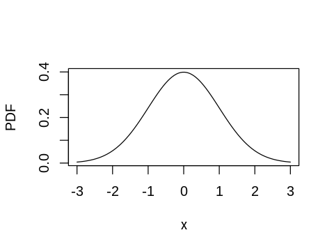
x <- seq(-3, 3, length.out = 100)
plot(x, dnorm(x), type="l", ylab="PDF")

CDF

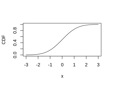
x <- seq(-3, 3, length.out = 100)
plot(x, pnorm(x), type="l", ylab="CDF")

Quantiles (inverse CDF)

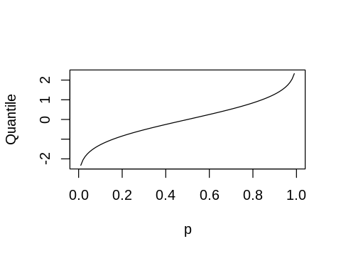
p = seq(0, 1, length.out = 101)
plot(p, qnorm(p), type="l", ylab="Quantile")

Point estimates

x <- rnorm(10)

x

1. -0.106124516091484
2. 1.51152199743894
3. -0.0946590384130976
4. 2.01842371387704
5. -0.062714099052421
6. 1.30486965422349
7. 2.28664539270111
8. -1.38886070111234
9. -0.278788766817371
10. -0.133321336393658

Mean

Manual calculation

sum(x)/length(x)

0.50569923003602

Using built-in function

mean(x)

0.50569923003602

Median

Manual calculation

x_sorted <- sort(x)

length(x)

10

Since there are an even number of observations, we need the average of the middle two data poitns

sum(x_sorted[5:6])/2

-0.0786865687327593

Using built-in function

median(x)

-0.0786865687327593

Quantiles

The mean is just the \(50^{th}\) percentile. We can use R to get any percentile we like.

quantile(x, 0.5)

50%: -0.0786865687327593

quantile(x, seq(0,1,length.out = 5))

0%

-1.38886070111234

25%

-0.126522131318115

50%

-0.0786865687327593

75%

1.45985891163508

100%

2.28664539270111

Exercise

Gene X is known to have a normal distribution with a mean of 100 units and a standard deviation of 15 units in the US population. With respect to this population,

• 1. What is the medan value for gene X?

100

100

• 2. What is the probability of finding a value of more than 130 for gene X if you pick a person at random?

m <- 100
s <- 15

1 - pnorm(130, m, s)

0.0227501319481792

• 3. If you measure gene X and find that it is in the 95th percentile for this population, what is the measured value?

qnorm(0.95, m, s)

124.672804404272

• 4. Find answers to questions (1), (2) and (3) by simulating 1 million people sampled from the US population. Do they agree with the theoretical calculated values?

n <- 1e6
x <- rnorm(n, m, s)

median(x)

100.020793858963

sum(x > 130)/n

0.022838

quantile(x, 0.95)

95%: 124.695020504446

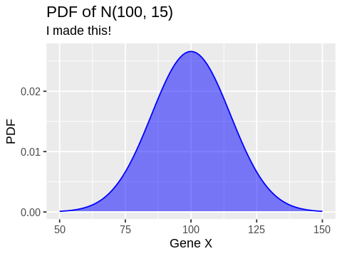
• 5. Plot the PDF of gene X using ggplot2 for values between 50 and 150. Give it a title of PDF of N(100, 15), a subtile of I made this!, and label the x-axis as Gene X and y-axis as PDF. Make the PDF blue, and fill the region under the curve blue with a transparency of 50%.

x <- 50:150
df <- data.frame(x=x, y=dnorm(x, m, s))
ggplot(df, aes(x=x, y=y)) +
geom_line(color='blue') +
geom_polygon(fill='blue', alpha=0.5) +
labs(title='PDF of N(100, 15)',
    subtitle='I made this!',
    x='Gene X',
    y='PDF')

Interval estimates

Confidence intervals

ci = 0.95

alpha = (1-ci)
n <- length(x)
m <- mean(x)
s <- sd(x)
se <- s/sqrt(n)
me <- qt(1-alpha/2, df=n-1) * se
c(m - me, m + me)

1. 94.215778757373
2. 105.784221242627

Note that confidence intervals get larger as the confidence required increases.

ci = 0.99

alpha = (1-ci)
n <- length(x)
m <- mean(x)
s <- sd(x)
se <- s/sqrt(n)
me <- qt(1-alpha/2, df=n-1) * se
c(m - me, m + me)

1. 92.3442793441823
2. 107.655720655818

Making a function

Review of R custom functions

f <- function(a, b=1) {
    a + b
}

f(2)

3

f(2,3)

5

f(b=4, a=1)

5

Exercise

Make a function called conf for calculating confidence intervals for the sample mean that takes two arguments

• x is the vector of sample values

• ci is the confidence interval with a default of 0.95

The funciton should return a vector of two numbers indicating the lwoer and upper limeit of the confidence interval

Check that it gives the same answer as the example above.

conf <- function(x, ci=0.95) {
   alpha = (1-ci)
    n <- length(x)
    m <- mean(x)
    s <- sd(x)
    se <- s/sqrt(n)
    me <- qt(1-alpha/2, df=n-1) * se
    c(m - me, m + me)
}

conf(x)

1. 94.215778757373
2. 105.784221242627

Coverage

In 1,000 experiments, we expect the true mean (0) to lie within the estimated 95% CIs 950 times.

n_expt <- 1000
n <- 10
cls <- t(replicate(n_expt, conf(rnorm(n))))

sum(cls[,1] < 0 & 0 < cls[,2])

960

Hypothesis testing

Binomial test

set.seed(123)

n = 50
tosses = sample(c('H', 'T'), n, replace=TRUE, prob=c(0.55, 0.45))
t = table(tosses)
t

tosses
 H  T
27 23

binom.test(table(tosses))

    Exact binomial test

data:  table(tosses)
number of successes = 27, number of trials = 50, p-value = 0.6718
alternative hypothesis: true probability of success is not equal to 0.5
95 percent confidence interval:
 0.3932420 0.6818508
sample estimates:
probability of success
                  0.54

set.seed(123)

n = 250
tosses = sample(c('H', 'T'), n, replace=TRUE, prob=c(0.55, 0.45))
t = table(tosses)
t

tosses
  H   T
139 111

binom.test(t)

    Exact binomial test

data:  t
number of successes = 139, number of trials = 250, p-value = 0.0875
alternative hypothesis: true probability of success is not equal to 0.5
95 percent confidence interval:
 0.4920569 0.6185995
sample estimates:
probability of success
                 0.556

What happens if we choose a one-sided test?

binom.test(t, alternative = "greater")

    Exact binomial test

data:  t
number of successes = 139, number of trials = 250, p-value = 0.04375
alternative hypothesis: true probability of success is greater than 0.5
95 percent confidence interval:
 0.5020197 1.0000000
sample estimates:
probability of success
                 0.556

binom.test(t, alternative = "less")

    Exact binomial test

data:  t
number of successes = 139, number of trials = 250, p-value = 0.9668
alternative hypothesis: true probability of success is less than 0.5
95 percent confidence interval:
 0.0000000 0.6089811
sample estimates:
probability of success
                 0.556

What happens if we change our null hypothesis?

binom.test(t, p = 0.55)

    Exact binomial test

data:  t
number of successes = 139, number of trials = 250, p-value = 0.8989
alternative hypothesis: true probability of success is not equal to 0.55
95 percent confidence interval:
 0.4920569 0.6185995
sample estimates:
probability of success
                 0.556

Two-sample model

Welch t-test

set.seed(123)

n <- 10
x1 <- rnorm(n, 0, 1)
x2 <- rnorm(n, 1, 1)

t.test(x1, x2)

    Welch Two Sample t-test

data:  x1 and x2
t = -2.5438, df = 17.872, p-value = 0.02044
alternative hypothesis: true difference in means is not equal to 0
95 percent confidence interval:
 -2.0710488 -0.1969438
sample estimates:
 mean of x  mean of y
0.07462564 1.20862196

Standard t-test

t.test(x1, x2, var.equal = TRUE)

    Two Sample t-test

data:  x1 and x2
t = -2.5438, df = 18, p-value = 0.02036
alternative hypothesis: true difference in means is not equal to 0
95 percent confidence interval:
 -2.0705694 -0.1974232
sample estimates:
 mean of x  mean of y
0.07462564 1.20862196

Power of t-test

d <- 1 # Effect size is ratio of difference in means to standard deviation

library(pwr)
pwr.t.test(d = d, sig.level = 0.05, power = 0.9)

gives output

     Two-sample t test power calculation

              n = 22.02109
              d = 1
      sig.level = 0.05
          power = 0.9
    alternative = two.sided

NOTE: n is number in *each* group

Interpretation of the power calculaiton

If we did many experiments with n=23 per group where the effect size is as specified and the test assumptions are valid, we expect that at least 90% of them will have a p-value less than the nominal significance level (0.05). If we used n=22 we would expect that just under 90% of the experiments will have a p-value less than the nomial significance level (0.05).

In particular notet that about 1-power of the experiments will fail to show a statistically significant p value even if the assumptionss are met (false negative).

n_expts <- 10000
n <- 22
alpha = 0.05
sum(replicate(n_expts, t.test(rnorm(n, 0, 1), rnorm(n, 1, 1))$p.value) < alpha)/n_expts

0.901

n_expts <- 10000
n <- 23
alpha = 0.05
sum(replicate(n_expts, t.test(rnorm(n, 0, 1), rnorm(n, 1, 1))$p.value) < alpha)/n_expts

0.9125

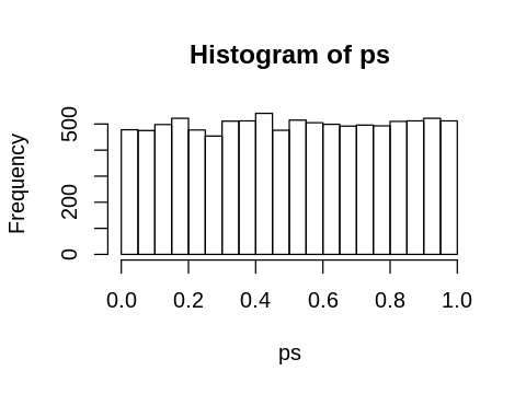
Distribution of p-values under the null is uniform

That meas that you expect \(\alpha\) of the experiments to be false positives.

n_expt <- 10000
n <- 50
ps <- replicate(n_expts, t.test(rnorm(n), rnorm(n))$p.value)

sum(ps < alpha)/n_expts

0.0478

hist(ps)

Paired and one-sample t-tests

A paired t-test is commonly used to evaluate if paired measuremetns (e..g. weight before and after a diet for the same person) has changed. The paired t-test is equivalent to a one-sample t-test that compares the difference in measurements for the paired values with a fixed number (usually 0).

x1 <- rnorm(10, 100, 15)
x2 <- rnorm(10, 100, 15)
delta <- x1 - x2

t.test(x1, x2, paired=TRUE)

    Paired t-test

data:  x1 and x2
t = -2.4618, df = 9, p-value = 0.03605
alternative hypothesis: true difference in means is not equal to 0
95 percent confidence interval:
 -12.3446069  -0.5215923
sample estimates:
mean of the differences
                -6.4331

t.test(delta, mu=0)

    One Sample t-test

data:  delta
t = -2.4618, df = 9, p-value = 0.03605
alternative hypothesis: true mean is not equal to 0
95 percent confidence interval:
 -12.3446069  -0.5215923
sample estimates:
mean of x
  -6.4331

Exercise

Suppose that the null hypotehsis is that there is no difference in the paired measurements and the standard deviation of the differene is 2.

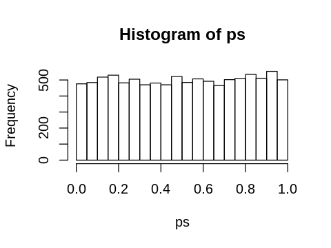
• Run a simulation for 100,000 experiments with n=25 per experiment to show the distributon of the p values using a paired or one -sample t-test under the null.

• If the significance level is 0.05, how many false positive results were observed?

n_expt <- 100000
n <- 25
s <- 2
ps <- replicate(n_expts, t.test(rnorm(10, 0, s), mu=0)$p.value)

hist(ps)

n <- 100000
s <- sqrt(2)
sd(rnorm(n, 0, s) - rnorm(n, 0, s))

2.00293039283011