DESeq2: Basic Differential Expression (DE) analysis
Objective: Carry out a basic set of DE analyses using DESeq2 and visualize the results
Load packages
[1]:
library(tidyverse)
library(DESeq2)
library(dendextend)
library(RColorBrewer)
Registered S3 methods overwritten by 'ggplot2':
  method         from
  [.quosures     rlang
  c.quosures     rlang
  print.quosures rlang
── Attaching packages ─────────────────────────────────────── tidyverse 1.2.1 ──
✔ ggplot2 3.1.1     ✔ purrr   0.3.2
✔ tibble  2.1.2     ✔ dplyr   0.8.1
✔ tidyr   0.8.3     ✔ stringr 1.4.0
✔ readr   1.3.1     ✔ forcats 0.4.0
── Conflicts ────────────────────────────────────────── tidyverse_conflicts() ──
✖ dplyr::filter() masks stats::filter()
✖ dplyr::lag()    masks stats::lag()
Loading required package: S4Vectors
Loading required package: stats4
Loading required package: BiocGenerics
Loading required package: parallel

Attaching package: ‘BiocGenerics’

The following objects are masked from ‘package:parallel’:

    clusterApply, clusterApplyLB, clusterCall, clusterEvalQ,
    clusterExport, clusterMap, parApply, parCapply, parLapply,
    parLapplyLB, parRapply, parSapply, parSapplyLB

The following objects are masked from ‘package:dplyr’:

    combine, intersect, setdiff, union

The following objects are masked from ‘package:stats’:

    IQR, mad, sd, var, xtabs

The following objects are masked from ‘package:base’:

    anyDuplicated, append, as.data.frame, basename, cbind, colnames,
    dirname, do.call, duplicated, eval, evalq, Filter, Find, get, grep,
    grepl, intersect, is.unsorted, lapply, Map, mapply, match, mget,
    order, paste, pmax, pmax.int, pmin, pmin.int, Position, rank,
    rbind, Reduce, rownames, sapply, setdiff, sort, table, tapply,
    union, unique, unsplit, which, which.max, which.min


Attaching package: ‘S4Vectors’

The following objects are masked from ‘package:dplyr’:

    first, rename

The following object is masked from ‘package:tidyr’:

    expand

The following object is masked from ‘package:base’:

    expand.grid

Loading required package: IRanges

Attaching package: ‘IRanges’

The following objects are masked from ‘package:dplyr’:

    collapse, desc, slice

The following object is masked from ‘package:purrr’:

    reduce

Loading required package: GenomicRanges
Loading required package: GenomeInfoDb
Loading required package: SummarizedExperiment
Loading required package: Biobase
Welcome to Bioconductor

    Vignettes contain introductory material; view with
    'browseVignettes()'. To cite Bioconductor, see
    'citation("Biobase")', and for packages 'citation("pkgname")'.

Loading required package: DelayedArray
Loading required package: matrixStats

Attaching package: ‘matrixStats’

The following objects are masked from ‘package:Biobase’:

    anyMissing, rowMedians

The following object is masked from ‘package:dplyr’:

    count

Loading required package: BiocParallel

Attaching package: ‘DelayedArray’

The following objects are masked from ‘package:matrixStats’:

    colMaxs, colMins, colRanges, rowMaxs, rowMins, rowRanges

The following object is masked from ‘package:purrr’:

    simplify

The following objects are masked from ‘package:base’:

    aperm, apply, rowsum


---------------------
Welcome to dendextend version 1.12.0
Type citation('dendextend') for how to cite the package.

Type browseVignettes(package = 'dendextend') for the package vignette.
The github page is: https://github.com/talgalili/dendextend/

Suggestions and bug-reports can be submitted at: https://github.com/talgalili/dendextend/issues
Or contact: <tal.galili@gmail.com>

        To suppress this message use:  suppressPackageStartupMessages(library(dendextend))
---------------------


Attaching package: ‘dendextend’

The following object is masked from ‘package:stats’:

    cutree
Load the 2019 pilot dds object from image file
[2]:
curdir <- "/home/jovyan/work/scratch/analysis_output"
imgdir <- file.path(curdir, "img")

imgfile <- file.path(imgdir, "pilotdds2019.RData")

imgfile

attach(imgfile)

tools::md5sum(imgfile)

### List the objects that have been attached
ls(2)

dds2019 <- dds2019

detach(pos = 2)
Check dimensions of the two objects
Inspect object & Slots of an S4 class
Let’s has a look at the object we have created.
[3]:
dds2019
class: DESeqDataSet
dim: 8499 24
metadata(1): version
assays(1): counts
rownames(8499): CNAG_00001 CNAG_00002 ... large_MTrRNA small_MTrRNA
rowData names(0):
colnames(24): 1_2019_P_M1 2_2019_P_M1 ... 23_2019_P_M1 24_2019_P_M1
colData names(22): Label sample_year ... RIN_normal_threshold
  RIN_lowered_threshold
see the class of dds object
[4]:
class(dds2019)
DESeqDataSet is a S4 object. Recall that a S4 object was taught when introducing bioconductor. Note that S4 objects allow users to wrap up multiple elements into a single variables where each element is called a slot.
[5]:
slotNames(dds2019)
- 'design'
- 'dispersionFunction'
- 'rowRanges'
- 'colData'
- 'assays'
- 'NAMES'
- 'elementMetadata'
- 'metadata'
The metadata (columnData) is stored in the slot colData
[6]:
dds2019@colData %>% as.data.frame %>% head(3)
| Label | sample_year | group | enrich_rep | RNA_sample_num | genotype | condition | libprep_person | enrichment_method | enrichment_short | ⋯ | i5_primer | i7_primer | library_num | bio_replicate | Nanodrop_260_280 | Nanodrop_260_230 | Nanodrop_concentration_ng_ul | Bioanalyzer_concentration_ng_ul | RIN_normal_threshold | RIN_lowered_threshold | |
|---|---|---|---|---|---|---|---|---|---|---|---|---|---|---|---|---|---|---|---|---|---|
| <chr> | <dbl> | <chr> | <dbl> | <dbl> | <fct> | <fct> | <chr> | <chr> | <chr> | ⋯ | <chr> | <chr> | <dbl> | <dbl> | <dbl> | <dbl> | <dbl> | <dbl> | <chr> | <dbl> | |
| 1_2019_P_M1 | 1_2019_P_M1 | 2019 | P | 1 | 1 | WT | pH4 | C | mRNA | M | ⋯ | i501 | i701 | 1 | 1 | 2.14 | 1.52 | 293 | 197 | N/A | 9.8 |
| 2_2019_P_M1 | 2_2019_P_M1 | 2019 | P | 1 | 2 | WT | pH4 | C | mRNA | M | ⋯ | i502 | i701 | 2 | 2 | 2.12 | 1.79 | 290 | 225 | N/A | 9.9 |
| 3_2019_P_M1 | 3_2019_P_M1 | 2019 | P | 1 | 3 | WT | pH4 | C | mRNA | M | ⋯ | i503 | i701 | 3 | 3 | 2.11 | 2.49 | 302 | 241 | N/A | 9.9 |
The design formula is stored in the slot design. The design holds the R formula which expresses how the counts depend on the variables in colData.
[7]:
dds2019@design
~condition + genotype
The first thing you may want to do is have a look at the raw counts you have imported. The DESeq2::counts function extracts a matrix of counts (with the genes along the rows and samples along the columns). Let us first verify the dimension of this matrix.
[8]:
dim(counts(dds2019))
- 8499
- 24
[9]:
head(counts(dds2019),3)
| 1_2019_P_M1 | 2_2019_P_M1 | 3_2019_P_M1 | 4_2019_P_M1 | 5_2019_P_M1 | 6_2019_P_M1 | 7_2019_P_M1 | 8_2019_P_M1 | 9_2019_P_M1 | 10_2019_P_M1 | ⋯ | 15_2019_P_M1 | 16_2019_P_M1 | 17_2019_P_M1 | 18_2019_P_M1 | 19_2019_P_M1 | 20_2019_P_M1 | 21_2019_P_M1 | 22_2019_P_M1 | 23_2019_P_M1 | 24_2019_P_M1 | |
|---|---|---|---|---|---|---|---|---|---|---|---|---|---|---|---|---|---|---|---|---|---|
| CNAG_00001 | 0 | 0 | 0 | 0 | 0 | 0 | 0 | 0 | 0 | 0 | ⋯ | 0 | 0 | 0 | 0 | 0 | 0 | 0 | 0 | 0 | 0 |
| CNAG_00002 | 158 | 204 | 149 | 176 | 161 | 148 | 172 | 169 | 124 | 119 | ⋯ | 216 | 224 | 234 | 338 | 191 | 201 | 192 | 166 | 202 | 235 |
| CNAG_00003 | 201 | 156 | 161 | 171 | 162 | 103 | 172 | 170 | 175 | 131 | ⋯ | 197 | 195 | 211 | 201 | 118 | 133 | 109 | 113 | 154 | 169 |
This slot returns gene specific information (it will be populated later)
[10]:
dds2019@dispersionFunction
function ()
NULL
Estimate Size Factors and Dispersion Parameters
You recall that DESeq requires that we have estimates for sample specific size factors and gene specific dispersion factors. More specifically, recall that DESeq models the count \(K_{ij}\) (gene \(i\), sample \(j\)) as negative binomial with mean \(\mu_{ij}\) and dispersion parameter \(\alpha_i\). Here \(\mu_{ij}=s_j q_{ij}\) where \(\log_2(q_{ij}) = \beta_{0i} + \beta_{1i} z_j\). Here \(s_j\) is the sample \(j\) specific size factor.
Summarize of notation - \(K_{ij}\) denotes the observed number of reads mapped to gene \(i\) for sample \(j\) - \(K_{ij}\) follows a negative binomial distribution with - Mean \(\mu_{ij}\) - Dispersion parameter \(\alpha_i\) - Modelling - \(K_{ij} \sim NB(\mu_{ij}, \alpha_i)\) - \(\mu_{ij} = s_{j}q_{ij}\) - \(s_j\) is sample \(j\) specific normalization constant - \(\log_2(q_{ij}) = \beta_{0i} + \beta_{1i} z_j\)
01 Size Factors
We begin by estimating the size factors \(s_1,\ldots,s_n\):
[11]:
dds2019 <- estimateSizeFactors(dds2019)
Now, compare the dds object to that of before applying the estimateSizeFactors() function. What has changed? What remains unchanged?
[12]:
dds2019
class: DESeqDataSet
dim: 8499 24
metadata(1): version
assays(1): counts
rownames(8499): CNAG_00001 CNAG_00002 ... large_MTrRNA small_MTrRNA
rowData names(0):
colnames(24): 1_2019_P_M1 2_2019_P_M1 ... 23_2019_P_M1 24_2019_P_M1
colData names(23): Label sample_year ... RIN_lowered_threshold
  sizeFactor
Note that there is a sizeFactor added to colData. Let’s look at it more carefully
``` > dds # (before estimateSizeFactors) class: DESeqDataSet class: DESeqDataSet dim: 8499 24 metadata(1): version assays(1): counts rownames(8499): CNAG_00001 CNAG_00002 … large_MTrRNA small_MTrRNA rowData names(0): colnames(24): 1_2019_P_M1 2_2019_P_M1 … 23_2019_P_M1 24_2019_P_M1 colData names(22): Label sample_year … RIN_normal_threshold RIN_lowered_threshold
dds # (after estimateSizeFactors) class: DESeqDataSet dim: 8499 24 metadata(1): version assays(1): counts rownames(8499): CNAG_00001 CNAG_00002 … large_MTrRNA small_MTrRNA rowData names(0): colnames(24): 1_2019_P_M1 2_2019_P_M1 … 23_2019_P_M1 24_2019_P_M1 colData names(23): Label sample_year … RIN_lowered_threshold sizeFactor
You can also get the size factors directly
[13]:
sizeFactors(dds2019)
- 1_2019_P_M1
- 1.5916393221245
- 2_2019_P_M1
- 1.65871103315141
- 3_2019_P_M1
- 1.51289455728943
- 4_2019_P_M1
- 1.41966861598247
- 5_2019_P_M1
- 1.43738473025559
- 6_2019_P_M1
- 1.23710002282889
- 7_2019_P_M1
- 1.40148291158442
- 8_2019_P_M1
- 1.44217254922035
- 9_2019_P_M1
- 1.17444094436861
- 10_2019_P_M1
- 1.07636468283386
- 11_2019_P_M1
- 1.04216270302148
- 12_2019_P_M1
- 0.971238282275506
- 13_2019_P_M1
- 0.770986843971703
- 14_2019_P_M1
- 0.752382049912615
- 15_2019_P_M1
- 0.717679610028228
- 16_2019_P_M1
- 0.897840290244175
- 17_2019_P_M1
- 0.89364164432414
- 18_2019_P_M1
- 0.931618100592125
- 19_2019_P_M1
- 0.749435710766038
- 20_2019_P_M1
- 0.775571527912074
- 21_2019_P_M1
- 0.583832529967166
- 22_2019_P_M1
- 0.634399759403834
- 23_2019_P_M1
- 0.755186085659437
- 24_2019_P_M1
- 0.808836405192349
It is preferable to limit the number of decimal places. Next show the size factors rounded to 3 decimal places
[14]:
round(sizeFactors(dds2019),3)
- 1_2019_P_M1
- 1.592
- 2_2019_P_M1
- 1.659
- 3_2019_P_M1
- 1.513
- 4_2019_P_M1
- 1.42
- 5_2019_P_M1
- 1.437
- 6_2019_P_M1
- 1.237
- 7_2019_P_M1
- 1.401
- 8_2019_P_M1
- 1.442
- 9_2019_P_M1
- 1.174
- 10_2019_P_M1
- 1.076
- 11_2019_P_M1
- 1.042
- 12_2019_P_M1
- 0.971
- 13_2019_P_M1
- 0.771
- 14_2019_P_M1
- 0.752
- 15_2019_P_M1
- 0.718
- 16_2019_P_M1
- 0.898
- 17_2019_P_M1
- 0.894
- 18_2019_P_M1
- 0.932
- 19_2019_P_M1
- 0.749
- 20_2019_P_M1
- 0.776
- 21_2019_P_M1
- 0.584
- 22_2019_P_M1
- 0.634
- 23_2019_P_M1
- 0.755
- 24_2019_P_M1
- 0.809
Summarize size factors
[15]:
summary(sizeFactors(dds2019))
  Min. 1st Qu.  Median    Mean 3rd Qu.    Max.
0.5838  0.7670  0.9514  1.0515  1.4060  1.6587
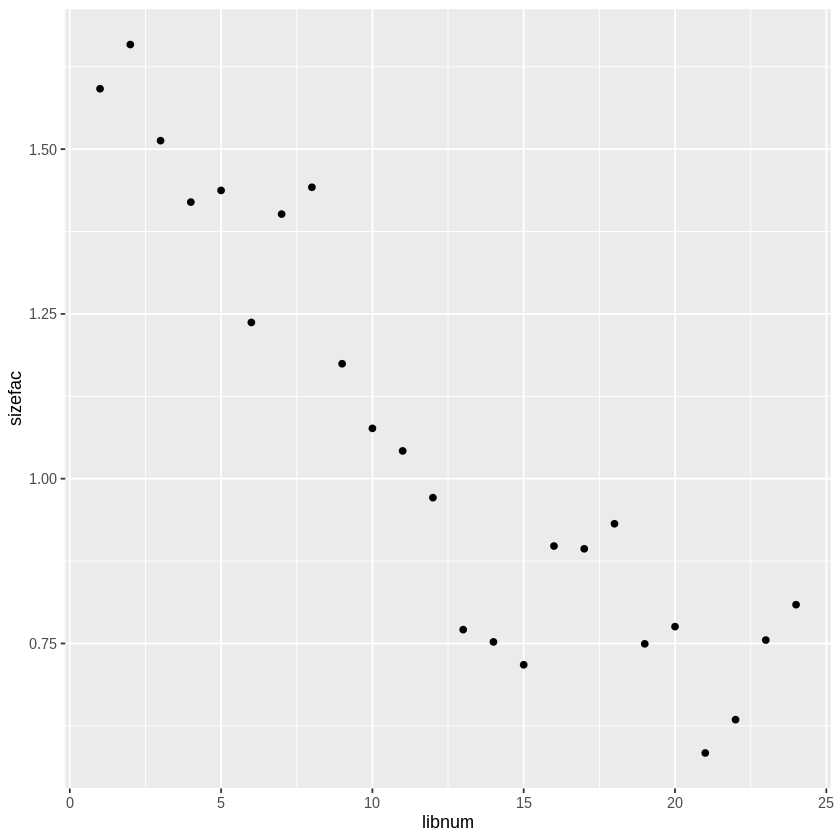
Do you see a trend?
[16]:
sizeFactors(dds2019) %>%
    as.data.frame %>%
        rownames_to_column %>%
            mutate(libnum = as.integer(str_remove(rowname, "_2019_P_M1"))) -> mydf

colnames(mydf)[2] <- "sizefac"

mydf
| rowname | sizefac | libnum |
|---|---|---|
| <chr> | <dbl> | <int> |
| 1_2019_P_M1 | 1.5916393 | 1 |
| 2_2019_P_M1 | 1.6587110 | 2 |
| 3_2019_P_M1 | 1.5128946 | 3 |
| 4_2019_P_M1 | 1.4196686 | 4 |
| 5_2019_P_M1 | 1.4373847 | 5 |
| 6_2019_P_M1 | 1.2371000 | 6 |
| 7_2019_P_M1 | 1.4014829 | 7 |
| 8_2019_P_M1 | 1.4421725 | 8 |
| 9_2019_P_M1 | 1.1744409 | 9 |
| 10_2019_P_M1 | 1.0763647 | 10 |
| 11_2019_P_M1 | 1.0421627 | 11 |
| 12_2019_P_M1 | 0.9712383 | 12 |
| 13_2019_P_M1 | 0.7709868 | 13 |
| 14_2019_P_M1 | 0.7523820 | 14 |
| 15_2019_P_M1 | 0.7176796 | 15 |
| 16_2019_P_M1 | 0.8978403 | 16 |
| 17_2019_P_M1 | 0.8936416 | 17 |
| 18_2019_P_M1 | 0.9316181 | 18 |
| 19_2019_P_M1 | 0.7494357 | 19 |
| 20_2019_P_M1 | 0.7755715 | 20 |
| 21_2019_P_M1 | 0.5838325 | 21 |
| 22_2019_P_M1 | 0.6343998 | 22 |
| 23_2019_P_M1 | 0.7551861 | 23 |
| 24_2019_P_M1 | 0.8088364 | 24 |
[17]:
ggplot(mydf, aes(x = libnum, y = sizefac)) + geom_point()
Now that the size factors have been estimated, we can get “normalized” counts (DESeq2 normalizes against size factor)
[18]:
# original counts for libraries 1 and 24
counts(dds2019)[1:5,c(1,24)]

# normalized count
counts(dds2019, normalize = TRUE)[1:5, c(1,24)]

# Size factor

sizeFactors(dds2019)[c(1,24)]
| 1_2019_P_M1 | 24_2019_P_M1 | |
|---|---|---|
| CNAG_00001 | 0 | 0 |
| CNAG_00002 | 158 | 235 |
| CNAG_00003 | 201 | 169 |
| CNAG_00004 | 904 | 523 |
| CNAG_00005 | 22 | 40 |
| 1_2019_P_M1 | 24_2019_P_M1 | |
|---|---|---|
| CNAG_00001 | 0.00000 | 0.00000 |
| CNAG_00002 | 99.26872 | 290.54083 |
| CNAG_00003 | 126.28489 | 208.94213 |
| CNAG_00004 | 567.96787 | 646.60789 |
| CNAG_00005 | 13.82223 | 49.45376 |
- 1_2019_P_M1
- 1.5916393221245
- 24_2019_P_M1
- 0.808836405192349
[19]:
# normalized manually using size factors for library 1
counts(dds2019)[1:5, 1] / sizeFactors(dds2019)[1]
- CNAG_00001
- 0
- CNAG_00002
- 99.2687211252757
- CNAG_00003
- 126.284892064433
- CNAG_00004
- 567.9678727674
- CNAG_00005
- 13.822226992127
[20]:
# normalized manually using size factors for library 24
counts(dds2019)[1:5, 24] / sizeFactors(dds2019)[24]
- CNAG_00001
- 0
- CNAG_00002
- 290.54082938331
- CNAG_00003
- 208.942128365019
- CNAG_00004
- 646.607888372217
- CNAG_00005
- 49.4537581929038
How do you get the raw counts for gene “GeneID: CNAG_05845”?
[21]:
counts(dds2019, normalize = TRUE)["CNAG_05845",]
- 1_2019_P_M1
- 1753.53797886484
- 2_2019_P_M1
- 1483.68217900155
- 3_2019_P_M1
- 1395.99946990619
- 4_2019_P_M1
- 1526.41255544016
- 5_2019_P_M1
- 1540.99313383281
- 6_2019_P_M1
- 1662.7596492127
- 7_2019_P_M1
- 1483.42871883441
- 8_2019_P_M1
- 1396.50418466832
- 9_2019_P_M1
- 1611.83072599508
- 10_2019_P_M1
- 1532.00864567435
- 11_2019_P_M1
- 1625.46596139805
- 12_2019_P_M1
- 1693.71412764532
- 13_2019_P_M1
- 1629.08097566201
- 14_2019_P_M1
- 1600.25083019968
- 15_2019_P_M1
- 1574.51874654145
- 16_2019_P_M1
- 1551.50087953968
- 17_2019_P_M1
- 1732.23798357198
- 18_2019_P_M1
- 1523.15632242235
- 19_2019_P_M1
- 1822.70471019287
- 20_2019_P_M1
- 1799.96293025118
- 21_2019_P_M1
- 1872.1121963887
- 22_2019_P_M1
- 1692.93885137862
- 23_2019_P_M1
- 1832.66088488836
- 24_2019_P_M1
- 1791.46239053794
02 Dispersion Parameters
Next, we get the dispersion factors \(\alpha_1,\ldots,\alpha_{m}\)
[22]:
dds2019 <- estimateDispersions(dds2019)
gene-wise dispersion estimates
mean-dispersion relationship
final dispersion estimates
metadata column names(0): - after:column names(9): baseMean baseVar ...[23]:
dds2019
class: DESeqDataSet
dim: 8499 24
metadata(1): version
assays(2): counts mu
rownames(8499): CNAG_00001 CNAG_00002 ... large_MTrRNA small_MTrRNA
rowData names(10): baseMean baseVar ... dispOutlier dispMAP
colnames(24): 1_2019_P_M1 2_2019_P_M1 ... 23_2019_P_M1 24_2019_P_M1
colData names(23): Label sample_year ... RIN_lowered_threshold
  sizeFactor
Can you notice the difference?
> dds (before dispersion)
class: DESeqDataSet
dim: 8499 24
metadata(1): version
assays(1): counts
rownames(8499): CNAG_00001 CNAG_00002 ... large_MTrRNA small_MTrRNA
rowData names(0):
colnames(24): 1_2019_P_M1 2_2019_P_M1 ... 23_2019_P_M1 24_2019_P_M1
colData names(23): Label sample_year ... RIN_lowered_threshold
  sizeFactor

> dds (after dispersion)
class: DESeqDataSet
dim: 8499 24
metadata(1): version
assays(2): counts mu
rownames(8499): CNAG_00001 CNAG_00002 ... large_MTrRNA small_MTrRNA
rowData names(10): baseMean baseVar ... dispOutlier dispMAP
colnames(24): 1_2019_P_M1 2_2019_P_M1 ... 23_2019_P_M1 24_2019_P_M1
colData names(23): Label sample_year ... RIN_lowered_threshold
  sizeFactor
Note that the dispersionfunction slot is now populated
[24]:
dds2019@dispersionFunction
structure(function (q)
coefs[1] + coefs[2]/q, coefficients = c(asymptDisp = 0.0141803487671824,
extraPois = 0.87630661036897), fitType = "parametric", varLogDispEsts = 0.902466256228483, dispPriorVar = 0.802549300169356)
We can extract the gene specific dispersion factors using dispersions(). Note that there will be one number per gene. We look at the first four genes (rounded to 4 decimal places)
[25]:
alphas <- dispersions(dds2019)
Verify that the number of dispersion factors equals the number of genes
[26]:
# number of disperion factors
length(alphas)
[27]:
round(alphas[1:4], 4)
- <NA>
- 0.0132
- 0.0231
- 0.0044
Extract the metadata using mcols() for the first four genes
Terms |
Description |
|---|---|
baseMean |
mean of normalized counts for all samples |
baseVar |
variance of normalized counts for all samples |
allZero |
all counts for a gene are zero |
dispGeneEst |
gene-wise estimates of dispersion |
dispFit |
fitted values of dispersion |
dispersion |
final estimate of dispersion |
dispIter |
number of iterations |
dispOut |
dispersion flagged as outlier |
dispMAP |
maximum a posteriori estimate |
[28]:
mcols(dds2019)[1:4,] %>% as.data.frame
| baseMean | baseVar | allZero | dispGeneEst | dispGeneIter | dispFit | dispersion | dispIter | dispOutlier | dispMAP | |
|---|---|---|---|---|---|---|---|---|---|---|
| <dbl> | <dbl> | <lgl> | <dbl> | <dbl> | <dbl> | <dbl> | <dbl> | <lgl> | <dbl> | |
| CNAG_00001 | 0.0000 | 0.000 | TRUE | NA | NA | NA | NA | NA | NA | NA |
| CNAG_00002 | 192.4564 | 8133.183 | FALSE | 0.012090962 | 9 | 0.01873362 | 0.013202310 | 9 | FALSE | 0.013202310 |
| CNAG_00003 | 164.9908 | 3089.489 | FALSE | 0.023820456 | 10 | 0.01949159 | 0.023065791 | 7 | FALSE | 0.023065791 |
| CNAG_00004 | 571.0547 | 1819.185 | FALSE | 0.003107148 | 5 | 0.01571489 | 0.004430586 | 12 | FALSE | 0.004430586 |
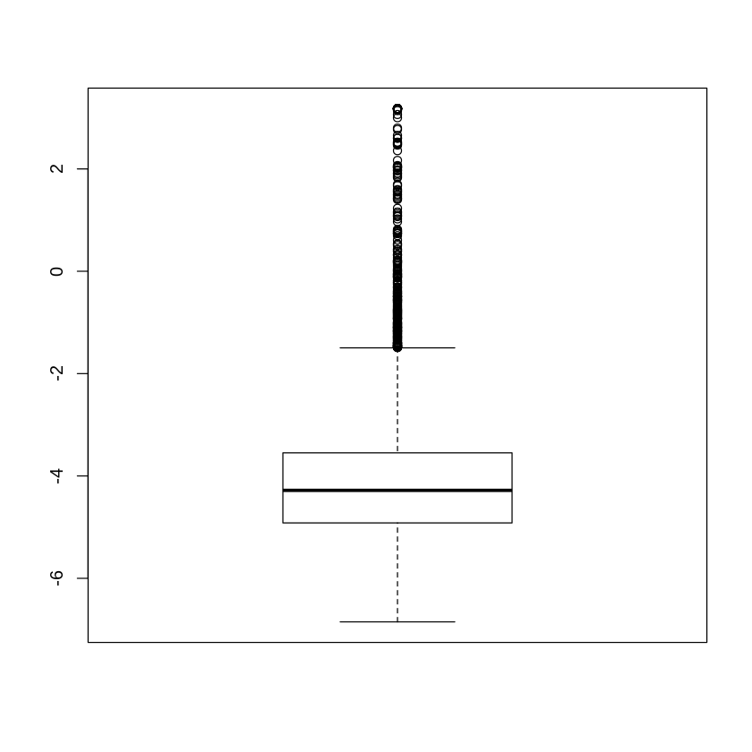
Summarize the dispersion factors using a box plot (may want to log transform)
[29]:
boxplot(log(dispersions(dds2019)))
Differential Expression Analysis
We can now conduct a differential expression analysis using the DESeq() function. Keep in mind that to get to this step, we first estimated the size factors and then the dispersion parameters.
[30]:
### Carry out DE analysis
ddsDE <- DESeq(dds2019)
using pre-existing size factors
estimating dispersions
found already estimated dispersions, replacing these
gene-wise dispersion estimates
mean-dispersion relationship
final dispersion estimates
fitting model and testing
[31]:
### Look at object
ddsDE
class: DESeqDataSet
dim: 8499 24
metadata(1): version
assays(4): counts mu H cooks
rownames(8499): CNAG_00001 CNAG_00002 ... large_MTrRNA small_MTrRNA
rowData names(26): baseMean baseVar ... deviance maxCooks
colnames(24): 1_2019_P_M1 2_2019_P_M1 ... 23_2019_P_M1 24_2019_P_M1
colData names(23): Label sample_year ... RIN_lowered_threshold
  sizeFactor
[32]:
### Look at some of the results
results(ddsDE)
log2 fold change (MLE): genotype WT vs sre1d
Wald test p-value: genotype WT vs sre1d
DataFrame with 8499 rows and 6 columns
                        baseMean     log2FoldChange              lfcSE
                       <numeric>          <numeric>          <numeric>
CNAG_00001                     0                 NA                 NA
CNAG_00002      192.456384076694 0.0459290105698189 0.0812849125012254
CNAG_00003      164.990819436254 0.0432979308487266  0.101045100070341
CNAG_00004      571.054651467718 0.0347715410374543 0.0464312203030827
CNAG_00005      28.7106195205257 -0.377056805602812  0.192347436642309
...                          ...                ...                ...
ENSRNA049551942                0                 NA                 NA
ENSRNA049551964                0                 NA                 NA
ENSRNA049551993                0                 NA                 NA
large_MTrRNA    5333.97356461621 -0.396337460272526   0.13434088145007
small_MTrRNA    1705.75472334291 -0.436802837852531  0.295538981353034
                             stat              pvalue                padj
                        <numeric>           <numeric>           <numeric>
CNAG_00001                     NA                  NA                  NA
CNAG_00002      0.565037337883909   0.572048368119426   0.675469542016723
CNAG_00003      0.428501043777338   0.668286373790347   0.756450803050288
CNAG_00004      0.748882773497678   0.453927864041203   0.566263547566551
CNAG_00005      -1.96029025488907  0.0499618744055703   0.094333851813714
...                           ...                 ...                 ...
ENSRNA049551942                NA                  NA                  NA
ENSRNA049551964                NA                  NA                  NA
ENSRNA049551993                NA                  NA                  NA
large_MTrRNA    -2.95023715785154 0.00317530091247218 0.00896807960414441
small_MTrRNA     -1.4779872213566   0.139411198621898   0.221714577729148
Note that currently, the model we have is an additive model, which does not include the interaction term of Media and Strain
Look at some of the results (tidy version)
[33]:
results(ddsDE, tidy = TRUE)
| row | baseMean | log2FoldChange | lfcSE | stat | pvalue | padj |
|---|---|---|---|---|---|---|
| <chr> | <dbl> | <dbl> | <dbl> | <dbl> | <dbl> | <dbl> |
| CNAG_00001 | 0.00000 | NA | NA | NA | NA | NA |
| CNAG_00002 | 192.45638 | 0.0459290106 | 0.08128491 | 0.565037338 | 5.720484e-01 | 6.754695e-01 |
| CNAG_00003 | 164.99082 | 0.0432979308 | 0.10104510 | 0.428501044 | 6.682864e-01 | 7.564508e-01 |
| CNAG_00004 | 571.05465 | 0.0347715410 | 0.04643122 | 0.748882773 | 4.539279e-01 | 5.662635e-01 |
| CNAG_00005 | 28.71062 | -0.3770568056 | 0.19234744 | -1.960290255 | 4.996187e-02 | 9.433385e-02 |
| CNAG_00006 | 3147.39964 | -0.1313696927 | 0.04955489 | -2.650993457 | 8.025540e-03 | 1.995982e-02 |
| CNAG_00007 | 1484.87545 | -0.2511214344 | 0.08051906 | -3.118782455 | 1.816000e-03 | 5.492473e-03 |
| CNAG_00008 | 938.01932 | -0.0095775568 | 0.04760749 | -0.201177504 | 8.405598e-01 | 8.873725e-01 |
| CNAG_00009 | 305.19881 | -0.1866458870 | 0.09952871 | -1.875296922 | 6.075189e-02 | 1.116044e-01 |
| CNAG_00010 | 989.04227 | 0.2991011506 | 0.06322330 | 4.730868797 | 2.235610e-06 | 1.474309e-05 |
| CNAG_00011 | 1001.75238 | -0.0150629941 | 0.08611946 | -0.174908133 | 8.611518e-01 | 9.032619e-01 |
| CNAG_00012 | 773.99385 | 0.1947487902 | 0.05765064 | 3.378085337 | 7.299243e-04 | 2.477973e-03 |
| CNAG_00013 | 485.75319 | -0.0002823069 | 0.07949652 | -0.003551185 | 9.971666e-01 | 9.974113e-01 |
| CNAG_00014 | 180.53988 | 0.0489307250 | 0.06795183 | 0.720079553 | 4.714760e-01 | 5.825377e-01 |
| CNAG_00015 | 318.87538 | -0.5225627661 | 0.04948141 | -10.560789734 | 4.528359e-26 | 6.591188e-24 |
| CNAG_00016 | 901.25567 | -0.1743972099 | 0.04458282 | -3.911758549 | 9.162649e-05 | 3.953666e-04 |
| CNAG_00017 | 184.65031 | 0.2501141367 | 0.08576066 | 2.916420444 | 3.540730e-03 | 9.829867e-03 |
| CNAG_00018 | 876.12980 | 0.0533671855 | 0.03737492 | 1.427887678 | 1.533242e-01 | 2.399204e-01 |
| CNAG_00019 | 1208.90542 | -0.0376199793 | 0.05412226 | -0.695092485 | 4.869973e-01 | 5.980888e-01 |
| CNAG_00020 | 968.39030 | 0.1633467817 | 0.06202149 | 2.633712498 | 8.445697e-03 | 2.079157e-02 |
| CNAG_00021 | 539.92676 | 0.3455959860 | 0.05392145 | 6.409249293 | 1.462379e-10 | 2.337226e-09 |
| CNAG_00022 | 746.84601 | -0.0338002495 | 0.06149652 | -0.549628633 | 5.825741e-01 | 6.837382e-01 |
| CNAG_00023 | 278.87826 | -1.4600937656 | 0.26611238 | -5.486756279 | 4.093813e-08 | 3.977196e-07 |
| CNAG_00024 | 7703.04647 | -0.1074959195 | 0.04323925 | -2.486072815 | 1.291615e-02 | 3.001984e-02 |
| CNAG_00025 | 2021.99612 | -0.0966388995 | 0.09609375 | -1.005673059 | 3.145729e-01 | 4.265652e-01 |
| CNAG_00026 | 2237.77134 | -0.2217950575 | 0.06090899 | -3.641417339 | 2.711412e-04 | 1.034194e-03 |
| CNAG_00027 | 425.60765 | 0.1226841378 | 0.06051990 | 2.027170038 | 4.264503e-02 | 8.258484e-02 |
| CNAG_00028 | 381.48552 | -0.1052942893 | 0.05837561 | -1.803737692 | 7.127244e-02 | 1.274834e-01 |
| CNAG_00029 | 52.66523 | -0.0698792034 | 0.10076540 | -0.693484135 | 4.880058e-01 | 5.990298e-01 |
| CNAG_00030 | 76.57328 | -0.3288112337 | 0.12296567 | -2.674008451 | 7.495056e-03 | 1.881006e-02 |
| ⋮ | ⋮ | ⋮ | ⋮ | ⋮ | ⋮ | ⋮ |
| ENSRNA049550980 | 0.000 | NA | NA | NA | NA | NA |
| ENSRNA049551037 | 0.000 | NA | NA | NA | NA | NA |
| ENSRNA049551063 | 0.000 | NA | NA | NA | NA | NA |
| ENSRNA049551074 | 0.000 | NA | NA | NA | NA | NA |
| ENSRNA049551126 | 0.000 | NA | NA | NA | NA | NA |
| ENSRNA049551197 | 0.000 | NA | NA | NA | NA | NA |
| ENSRNA049551244 | 0.000 | NA | NA | NA | NA | NA |
| ENSRNA049551269 | 0.000 | NA | NA | NA | NA | NA |
| ENSRNA049551298 | 0.000 | NA | NA | NA | NA | NA |
| ENSRNA049551337 | 0.000 | NA | NA | NA | NA | NA |
| ENSRNA049551365 | 0.000 | NA | NA | NA | NA | NA |
| ENSRNA049551391 | 0.000 | NA | NA | NA | NA | NA |
| ENSRNA049551484 | 0.000 | NA | NA | NA | NA | NA |
| ENSRNA049551550 | 0.000 | NA | NA | NA | NA | NA |
| ENSRNA049551574 | 0.000 | NA | NA | NA | NA | NA |
| ENSRNA049551598 | 0.000 | NA | NA | NA | NA | NA |
| ENSRNA049551636 | 0.000 | NA | NA | NA | NA | NA |
| ENSRNA049551673 | 0.000 | NA | NA | NA | NA | NA |
| ENSRNA049551717 | 0.000 | NA | NA | NA | NA | NA |
| ENSRNA049551745 | 0.000 | NA | NA | NA | NA | NA |
| ENSRNA049551774 | 0.000 | NA | NA | NA | NA | NA |
| ENSRNA049551798 | 0.000 | NA | NA | NA | NA | NA |
| ENSRNA049551814 | 0.000 | NA | NA | NA | NA | NA |
| ENSRNA049551862 | 0.000 | NA | NA | NA | NA | NA |
| ENSRNA049551899 | 0.000 | NA | NA | NA | NA | NA |
| ENSRNA049551942 | 0.000 | NA | NA | NA | NA | NA |
| ENSRNA049551964 | 0.000 | NA | NA | NA | NA | NA |
| ENSRNA049551993 | 0.000 | NA | NA | NA | NA | NA |
| large_MTrRNA | 5333.974 | -0.3963375 | 0.1343409 | -2.950237 | 0.003175301 | 0.00896808 |
| small_MTrRNA | 1705.755 | -0.4368028 | 0.2955390 | -1.477987 | 0.139411199 | 0.22171458 |
We can get the results for the differential expression analysis using results(). Here, we can compare two group of samples specified by the contrast. (If not, the default contrast would be the last term in your additive model design(dds)).
[34]:
# DE with respect to condition
myres_condition4v8 <- results(ddsDE, contrast = c("condition", "pH4", "pH8"))
myres_condition4v8
log2 fold change (MLE): condition pH4 vs pH8
Wald test p-value: condition pH4 vs pH8
DataFrame with 8499 rows and 6 columns
                        baseMean      log2FoldChange              lfcSE
                       <numeric>           <numeric>          <numeric>
CNAG_00001                     0                  NA                 NA
CNAG_00002      192.456384076694   -1.34351851614176 0.0813854454817818
CNAG_00003      164.990819436254  -0.831905577724638  0.101018400723969
CNAG_00004      571.054651467718 -0.0871138906737344 0.0465166816365353
CNAG_00005      28.7106195205257   -1.29275886849841  0.192729463777133
...                          ...                 ...                ...
ENSRNA049551942                0                  NA                 NA
ENSRNA049551964                0                  NA                 NA
ENSRNA049551993                0                  NA                 NA
large_MTrRNA    5333.97356461621  -0.948564278537808  0.134340883270906
small_MTrRNA    1705.75472334291  -0.691472418621256  0.295538979277226
                             stat               pvalue                 padj
                        <numeric>            <numeric>            <numeric>
CNAG_00001                     NA                   NA                   NA
CNAG_00002      -16.5080931631996 3.20862403991611e-61 2.87085560366149e-60
CNAG_00003      -8.23518855735805 1.79275046151211e-16 4.79576928512805e-16
CNAG_00004      -1.87274516601186   0.0611035831980367    0.074895534834165
CNAG_00005      -6.70763485334717 1.97804137561036e-11 4.32020773113613e-11
...                           ...                  ...                  ...
ENSRNA049551942                NA                   NA                   NA
ENSRNA049551964                NA                   NA                   NA
ENSRNA049551993                NA                   NA                   NA
large_MTrRNA    -7.06087570248421 1.65456549165796e-12 3.75246614426935e-12
small_MTrRNA    -2.33969955608675   0.0192992582107572   0.0250291573072207
[35]:
# DE with respect to condition (flip order)
myres_condition8v4 <- results(ddsDE, contrast = c("condition", "pH8", "pH4"))
myres_condition8v4
log2 fold change (MLE): condition pH8 vs pH4
Wald test p-value: condition pH8 vs pH4
DataFrame with 8499 rows and 6 columns
                        baseMean     log2FoldChange              lfcSE
                       <numeric>          <numeric>          <numeric>
CNAG_00001                     0                 NA                 NA
CNAG_00002      192.456384076694   1.34351851614176 0.0813854454817818
CNAG_00003      164.990819436254  0.831905577724638  0.101018400723969
CNAG_00004      571.054651467718 0.0871138906737344 0.0465166816365353
CNAG_00005      28.7106195205257   1.29275886849841  0.192729463777133
...                          ...                ...                ...
ENSRNA049551942                0                 NA                 NA
ENSRNA049551964                0                 NA                 NA
ENSRNA049551993                0                 NA                 NA
large_MTrRNA    5333.97356461621  0.948564278537808  0.134340883270906
small_MTrRNA    1705.75472334291  0.691472418621256  0.295538979277226
                            stat               pvalue                 padj
                       <numeric>            <numeric>            <numeric>
CNAG_00001                    NA                   NA                   NA
CNAG_00002      16.5080931631996 3.20862403991611e-61 2.87085560366149e-60
CNAG_00003      8.23518855735805 1.79275046151211e-16 4.79576928512805e-16
CNAG_00004      1.87274516601186   0.0611035831980367    0.074895534834165
CNAG_00005      6.70763485334717 1.97804137561036e-11 4.32020773113613e-11
...                          ...                  ...                  ...
ENSRNA049551942               NA                   NA                   NA
ENSRNA049551964               NA                   NA                   NA
ENSRNA049551993               NA                   NA                   NA
large_MTrRNA    7.06087570248421 1.65456549165796e-12 3.75246614426935e-12
small_MTrRNA    2.33969955608675   0.0192992582107572   0.0250291573072207
[36]:
### DE with respect to genotype
myres_strainvWT <- results(ddsDE, contrast = c("genotype", "sre1d", "WT"))
myres_strainvWT
log2 fold change (MLE): genotype sre1d vs WT
Wald test p-value: genotype sre1d vs WT
DataFrame with 8499 rows and 6 columns
                        baseMean      log2FoldChange              lfcSE
                       <numeric>           <numeric>          <numeric>
CNAG_00001                     0                  NA                 NA
CNAG_00002      192.456384076694 -0.0459290105698189 0.0812849125012254
CNAG_00003      164.990819436254 -0.0432979308487266  0.101045100070341
CNAG_00004      571.054651467718 -0.0347715410374543 0.0464312203030827
CNAG_00005      28.7106195205257   0.377056805602812  0.192347436642309
...                          ...                 ...                ...
ENSRNA049551942                0                  NA                 NA
ENSRNA049551964                0                  NA                 NA
ENSRNA049551993                0                  NA                 NA
large_MTrRNA    5333.97356461621   0.396337460272526   0.13434088145007
small_MTrRNA    1705.75472334291   0.436802837852531  0.295538981353034
                              stat              pvalue                padj
                         <numeric>           <numeric>           <numeric>
CNAG_00001                      NA                  NA                  NA
CNAG_00002      -0.565037337883909   0.572048368119426   0.675469542016723
CNAG_00003      -0.428501043777338   0.668286373790347   0.756450803050288
CNAG_00004      -0.748882773497678   0.453927864041203   0.566263547566551
CNAG_00005        1.96029025488907  0.0499618744055703   0.094333851813714
...                            ...                 ...                 ...
ENSRNA049551942                 NA                  NA                  NA
ENSRNA049551964                 NA                  NA                  NA
ENSRNA049551993                 NA                  NA                  NA
large_MTrRNA      2.95023715785154 0.00317530091247218 0.00896807960414441
small_MTrRNA       1.4779872213566   0.139411198621898   0.221714577729148
Let’s look at the results for the first four genes
[37]:
### Tidy the results
myres_condition8v4 <- results(ddsDE, contrast = c("condition", "pH8", "pH4"), tidy = TRUE)
myres_condition8v4
| row | baseMean | log2FoldChange | lfcSE | stat | pvalue | padj |
|---|---|---|---|---|---|---|
| <chr> | <dbl> | <dbl> | <dbl> | <dbl> | <dbl> | <dbl> |
| CNAG_00001 | 0.00000 | NA | NA | NA | NA | NA |
| CNAG_00002 | 192.45638 | 1.343518516 | 0.08138545 | 16.5080932 | 3.208624e-61 | 2.870856e-60 |
| CNAG_00003 | 164.99082 | 0.831905578 | 0.10101840 | 8.2351886 | 1.792750e-16 | 4.795769e-16 |
| CNAG_00004 | 571.05465 | 0.087113891 | 0.04651668 | 1.8727452 | 6.110358e-02 | 7.489553e-02 |
| CNAG_00005 | 28.71062 | 1.292758868 | 0.19272946 | 6.7076349 | 1.978041e-11 | 4.320208e-11 |
| CNAG_00006 | 3147.39964 | -0.139327775 | 0.04956000 | -2.8112951 | 4.934250e-03 | 6.756102e-03 |
| CNAG_00007 | 1484.87545 | -0.747920328 | 0.08053624 | -9.2867544 | 1.590647e-20 | 4.927921e-20 |
| CNAG_00008 | 938.01932 | -0.079110196 | 0.04765929 | -1.6599115 | 9.693226e-02 | 1.159517e-01 |
| CNAG_00009 | 305.19881 | -0.558838066 | 0.09968395 | -5.6060989 | 2.069377e-08 | 3.933651e-08 |
| CNAG_00010 | 989.04227 | 0.537893668 | 0.06321490 | 8.5089694 | 1.754861e-17 | 4.868574e-17 |
| CNAG_00011 | 1001.75238 | -2.148894367 | 0.08634115 | -24.8884142 | 9.932146e-137 | 2.998405e-135 |
| CNAG_00012 | 773.99385 | 0.161412817 | 0.05766095 | 2.7993437 | 5.120661e-03 | 6.994889e-03 |
| CNAG_00013 | 485.75319 | -0.722966497 | 0.07965037 | -9.0767500 | 1.118652e-19 | 3.374959e-19 |
| CNAG_00014 | 180.53988 | -0.295886560 | 0.06870554 | -4.3065895 | 1.657908e-05 | 2.684468e-05 |
| CNAG_00015 | 318.87538 | -0.328599588 | 0.05019105 | -6.5469752 | 5.871409e-11 | 1.252823e-10 |
| CNAG_00016 | 901.25567 | 0.312717596 | 0.04460378 | 7.0110118 | 2.366008e-12 | 5.340717e-12 |
| CNAG_00017 | 184.65031 | 0.316683243 | 0.08573971 | 3.6935425 | 2.211516e-04 | 3.341873e-04 |
| CNAG_00018 | 876.12980 | 0.155211001 | 0.03742605 | 4.1471376 | 3.366577e-05 | 5.348074e-05 |
| CNAG_00019 | 1208.90542 | 0.747123679 | 0.05412045 | 13.8048310 | 2.383308e-43 | 1.414883e-42 |
| CNAG_00020 | 968.39030 | -0.470164125 | 0.06206999 | -7.5747418 | 3.598425e-14 | 8.737196e-14 |
| CNAG_00021 | 539.92676 | 0.007922036 | 0.05395599 | 0.1468240 | 8.832709e-01 | 8.975865e-01 |
| CNAG_00022 | 746.84601 | 0.020299074 | 0.06152583 | 0.3299277 | 7.414546e-01 | 7.689054e-01 |
| CNAG_00023 | 278.87826 | 0.232063963 | 0.26610452 | 0.8720782 | 3.831657e-01 | 4.210277e-01 |
| CNAG_00024 | 7703.04647 | 0.997043384 | 0.04323929 | 23.0587381 | 1.202071e-117 | 2.760023e-116 |
| CNAG_00025 | 2021.99612 | 0.881055403 | 0.09609371 | 9.1687104 | 4.787115e-20 | 1.463607e-19 |
| CNAG_00026 | 2237.77134 | 0.167433512 | 0.06091140 | 2.7488043 | 5.981308e-03 | 8.132384e-03 |
| CNAG_00027 | 425.60765 | -0.929646998 | 0.06112216 | -15.2096555 | 3.051445e-52 | 2.273522e-51 |
| CNAG_00028 | 381.48552 | -0.817422940 | 0.05910049 | -13.8310684 | 1.655433e-43 | 9.892547e-43 |
| CNAG_00029 | 52.66523 | -3.316030881 | 0.16631275 | -19.9385244 | 1.885448e-88 | 2.729713e-87 |
| CNAG_00030 | 76.57328 | -1.103647498 | 0.12592110 | -8.7645955 | 1.874484e-18 | 5.414216e-18 |
| ⋮ | ⋮ | ⋮ | ⋮ | ⋮ | ⋮ | ⋮ |
| ENSRNA049550980 | 0.000 | NA | NA | NA | NA | NA |
| ENSRNA049551037 | 0.000 | NA | NA | NA | NA | NA |
| ENSRNA049551063 | 0.000 | NA | NA | NA | NA | NA |
| ENSRNA049551074 | 0.000 | NA | NA | NA | NA | NA |
| ENSRNA049551126 | 0.000 | NA | NA | NA | NA | NA |
| ENSRNA049551197 | 0.000 | NA | NA | NA | NA | NA |
| ENSRNA049551244 | 0.000 | NA | NA | NA | NA | NA |
| ENSRNA049551269 | 0.000 | NA | NA | NA | NA | NA |
| ENSRNA049551298 | 0.000 | NA | NA | NA | NA | NA |
| ENSRNA049551337 | 0.000 | NA | NA | NA | NA | NA |
| ENSRNA049551365 | 0.000 | NA | NA | NA | NA | NA |
| ENSRNA049551391 | 0.000 | NA | NA | NA | NA | NA |
| ENSRNA049551484 | 0.000 | NA | NA | NA | NA | NA |
| ENSRNA049551550 | 0.000 | NA | NA | NA | NA | NA |
| ENSRNA049551574 | 0.000 | NA | NA | NA | NA | NA |
| ENSRNA049551598 | 0.000 | NA | NA | NA | NA | NA |
| ENSRNA049551636 | 0.000 | NA | NA | NA | NA | NA |
| ENSRNA049551673 | 0.000 | NA | NA | NA | NA | NA |
| ENSRNA049551717 | 0.000 | NA | NA | NA | NA | NA |
| ENSRNA049551745 | 0.000 | NA | NA | NA | NA | NA |
| ENSRNA049551774 | 0.000 | NA | NA | NA | NA | NA |
| ENSRNA049551798 | 0.000 | NA | NA | NA | NA | NA |
| ENSRNA049551814 | 0.000 | NA | NA | NA | NA | NA |
| ENSRNA049551862 | 0.000 | NA | NA | NA | NA | NA |
| ENSRNA049551899 | 0.000 | NA | NA | NA | NA | NA |
| ENSRNA049551942 | 0.000 | NA | NA | NA | NA | NA |
| ENSRNA049551964 | 0.000 | NA | NA | NA | NA | NA |
| ENSRNA049551993 | 0.000 | NA | NA | NA | NA | NA |
| large_MTrRNA | 5333.974 | 0.9485643 | 0.1343409 | 7.060876 | 1.654565e-12 | 3.752466e-12 |
| small_MTrRNA | 1705.755 | 0.6914724 | 0.2955390 | 2.339700 | 1.929926e-02 | 2.502916e-02 |
[38]:
### Tidy the results for DE with respect to condition
### Results are sorted in ascending order by adjusted p-value
### Here ph4 is the reference level
### log2FC > 0 suggests that higher pH (pH8) is associated with increased expression
### log2FC < 0 suggests that higher pH (pH8) is associated with lower expression
myres_condition8v4 <- results(ddsDE, contrast = c("condition", "pH8", "pH4"), tidy = TRUE)

myres_condition8v4 %>%
    arrange(desc(-padj)) %>%
        head(10)
| row | baseMean | log2FoldChange | lfcSE | stat | pvalue | padj |
|---|---|---|---|---|---|---|
| <chr> | <dbl> | <dbl> | <dbl> | <dbl> | <dbl> | <dbl> |
| CNAG_00275 | 1072.9219 | -4.048106 | 0.10667356 | -37.94854 | 0 | 0 |
| CNAG_00309 | 539.1312 | -3.331524 | 0.08444635 | -39.45137 | 0 | 0 |
| CNAG_00409 | 1093.4775 | -5.030655 | 0.07452918 | -67.49913 | 0 | 0 |
| CNAG_00531 | 15371.8856 | 3.563691 | 0.05663035 | 62.92900 | 0 | 0 |
| CNAG_00601 | 506.4752 | 4.661577 | 0.09625726 | 48.42832 | 0 | 0 |
| CNAG_00897 | 12255.8281 | 4.856924 | 0.07970883 | 60.93332 | 0 | 0 |
| CNAG_01272 | 49334.5209 | 1.961009 | 0.04521777 | 43.36812 | 0 | 0 |
| CNAG_01275 | 2534.1015 | 2.273088 | 0.04888985 | 46.49406 | 0 | 0 |
| CNAG_01344 | 3528.6160 | -1.582122 | 0.04028591 | -39.27234 | 0 | 0 |
| CNAG_01713 | 9652.4535 | 2.016486 | 0.05310869 | 37.96904 | 0 | 0 |
Visualize DE effect
Looking at the results for these two genes:
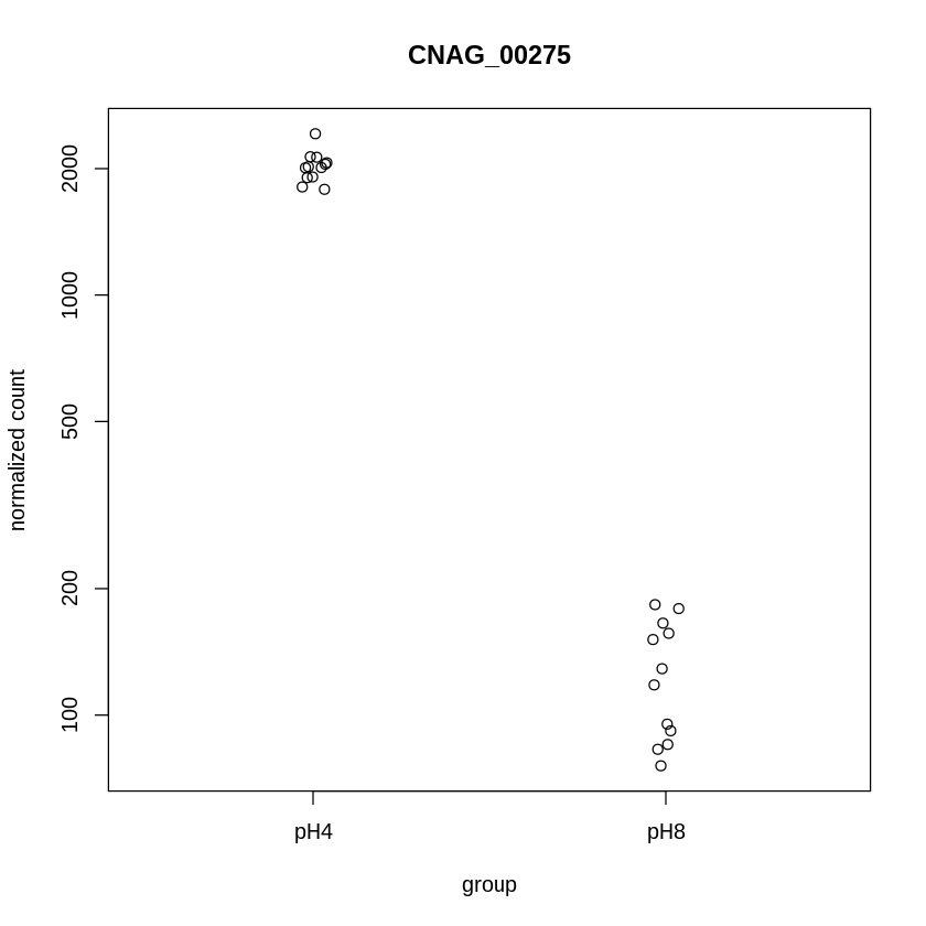
The estimated log2FC for CNAG_00275 is negative. We will verify visually that ph8, compared to pH4, is associated with lower expression
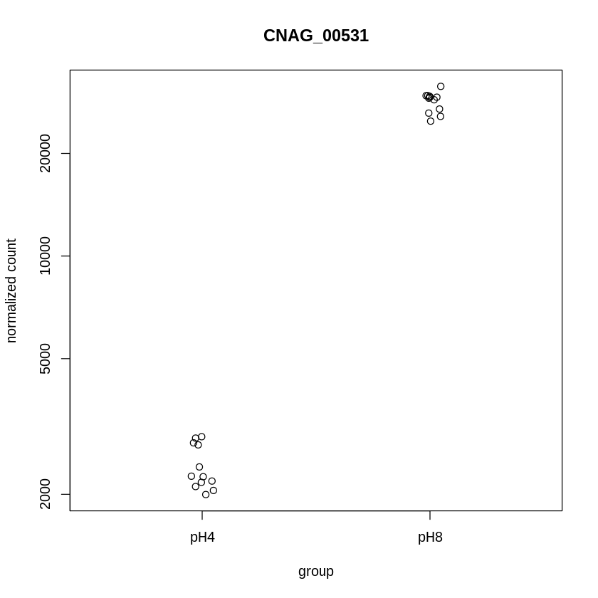
The estimated log2FC for CNAG_00531 is positive. We will verify visually that ph8, compared to pH4, is associated with higher expression
[39]:
results(ddsDE, tidy = TRUE) %>%
    filter(row %in% c("CNAG_00275","CNAG_00531"))
| row | baseMean | log2FoldChange | lfcSE | stat | pvalue | padj |
|---|---|---|---|---|---|---|
| <chr> | <dbl> | <dbl> | <dbl> | <dbl> | <dbl> | <dbl> |
| CNAG_00275 | 1072.922 | -0.3268490 | 0.10536149 | -3.102167 | 0.0019210943 | 0.005769654 |
| CNAG_00531 | 15371.886 | 0.1902424 | 0.05662427 | 3.359733 | 0.0007801794 | 0.002625616 |
[40]:
### This dot plot verify visually that exposure to ph8, compared to pH4,  is associated with lower expression
plotCounts(dds2019, "CNAG_00275", intgroup = "condition")
[41]:
### This dot plot verify visually that exposure to ph8, compared to pH4,  is associated with higher expression
plotCounts(dds2019, "CNAG_00531", intgroup = "condition")
Volcano plot
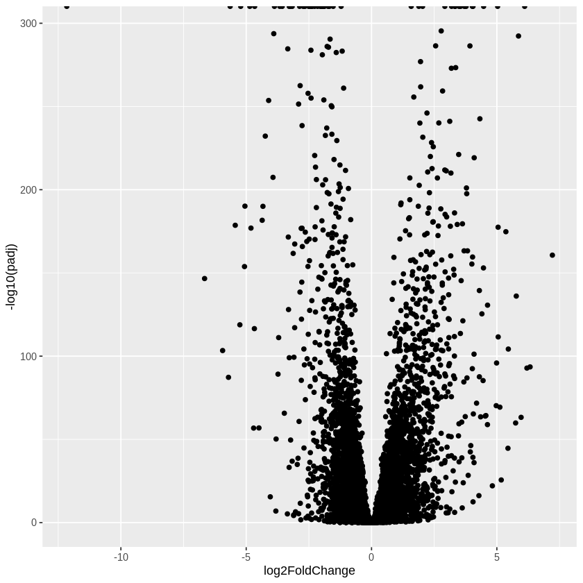
[42]:
### Volcano plot for con effect
ggplot(results(ddsDE, contrast = c("condition", "pH4", "pH8"), tidy = TRUE),
       aes(x = log2FoldChange, y = -log10(padj))) + geom_point()
Warning message:
“Removed 348 rows containing missing values (geom_point).”
[43]:
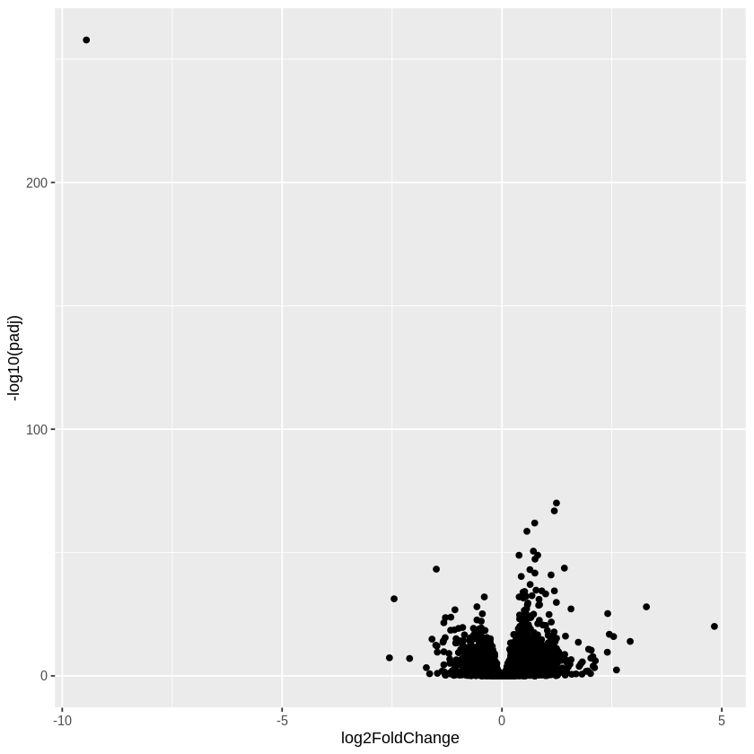
### Genotype Effect
ggplot(results(ddsDE, contrast = c("genotype", "sre1d", "WT"), tidy = TRUE),
       aes(x = log2FoldChange, y = -log10(padj))) + geom_point()
Warning message:
“Removed 348 rows containing missing values (geom_point).”
Clustering
Regularized log transformation
The regularized log transform can be obtained using the rlog() function. Note that an important argument for this function is blind (TRUE by default). The default “blinds” the normalization to the design. This is very important so as to not bias the analyses (e.g. class discovery)
[44]:
rld <- rlog(dds2019, blind = TRUE)
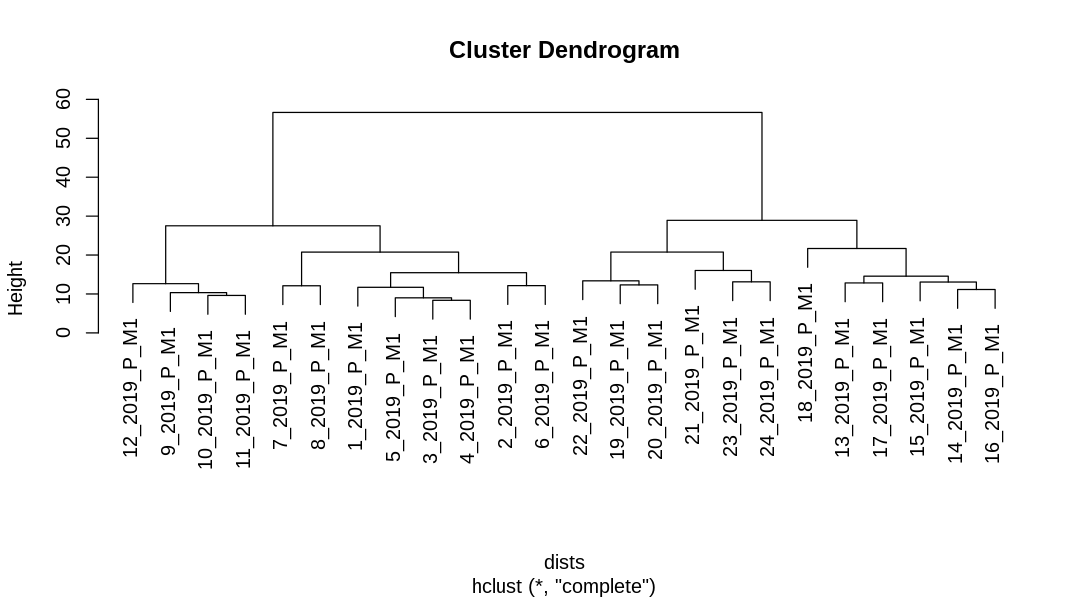
Dendrogram of samples: showing strain & media of each sample
Hierarchical clustering using rlog transformation
[45]:
options(repr.plot.width = 9, repr.plot.height = 5)
dists <- dist(t(assay(rld)))
plot(hclust(dists))
Store the dendrogram of samples using hierarchical clustering
[46]:
assay(rld) %>%
    t() %>%
    dist %>%
    hclust(method = "complete") %>%
    as.dendrogram ->
    mydend
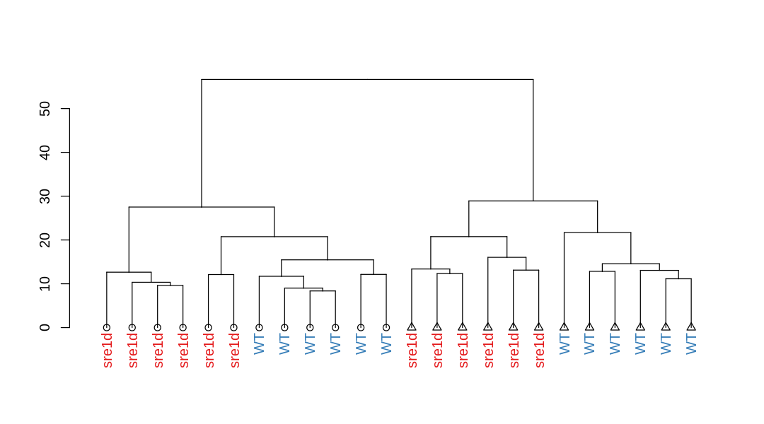
Dendrogram of samples: showing strain of each sample
[47]:
dendplot <- function(mydend, columndata, labvar, colvar, pchvar) {
    cols <- factor(columndata[[colvar]][order.dendrogram(mydend)])
    collab <- brewer.pal(max(3,nlevels(cols)),"Set1")[cols]
    pchs <- factor(columndata[[pchvar]][order.dendrogram(mydend)])
    pchlab <- seq_len(nlevels(pchs))[pchs]
    lablab <- columndata[[labvar]][order.dendrogram(mydend)]

    mydend %>%
        set("labels_cex",1) %>%
        set("labels_col",collab) %>%
        set("leaves_pch",pchlab) %>%
        set("labels", lablab)
}
[48]:
options(repr.plot.width = 9, repr.plot.height = 5)
dendplot(mydend, dds2019@colData,
         "genotype",    # variable that show in label
         "genotype",    # variable that define color
         "condition") %>% # variable that define shape of points
    plot
Dendrogram of samples: showing media of each sample
Customize presentation
[49]:
### Merge gene expression with meta data
myDEplotData <- function(mydds, geneid, mergelab) {
    counts(mydds, normalize = TRUE) %>%
        as_tibble(rownames="gene") %>%
        filter(gene == geneid) %>%
        gather(Label, geneexp, -gene) %>%
        select(-gene) -> genedat

    colData(mydds) %>%
        as.data.frame %>%
        as_tibble %>%
        full_join(genedat, by = mergelab) -> genedat

    return(genedat)
}

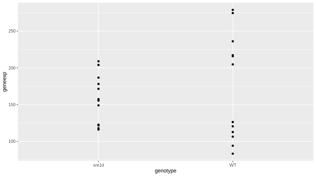
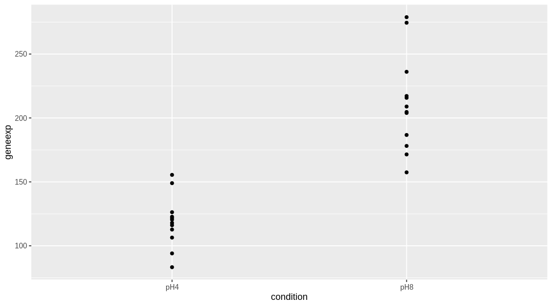
myDEplotData(dds2019, "CNAG_00003", "Label")[,c("Label", "genotype", "condition" , "geneexp")]
| Label | genotype | condition | geneexp |
|---|---|---|---|
| <chr> | <fct> | <fct> | <dbl> |
| 1_2019_P_M1 | WT | pH4 | 126.28489 |
| 2_2019_P_M1 | WT | pH4 | 94.04893 |
| 3_2019_P_M1 | WT | pH4 | 106.41852 |
| 4_2019_P_M1 | WT | pH4 | 120.45064 |
| 5_2019_P_M1 | WT | pH4 | 112.70469 |
| 6_2019_P_M1 | WT | pH4 | 83.25923 |
| 7_2019_P_M1 | sre1d | pH4 | 122.72715 |
| 8_2019_P_M1 | sre1d | pH4 | 117.87771 |
| 9_2019_P_M1 | sre1d | pH4 | 149.00707 |
| 10_2019_P_M1 | sre1d | pH4 | 121.70596 |
| 11_2019_P_M1 | sre1d | pH4 | 116.10471 |
| 12_2019_P_M1 | sre1d | pH4 | 155.47163 |
| 13_2019_P_M1 | WT | pH8 | 278.86338 |
| 14_2019_P_M1 | WT | pH8 | 204.68325 |
| 15_2019_P_M1 | WT | pH8 | 274.49575 |
| 16_2019_P_M1 | WT | pH8 | 217.18785 |
| 17_2019_P_M1 | WT | pH8 | 236.11254 |
| 18_2019_P_M1 | WT | pH8 | 215.75364 |
| 19_2019_P_M1 | sre1d | pH8 | 157.45180 |
| 20_2019_P_M1 | sre1d | pH8 | 171.48644 |
| 21_2019_P_M1 | sre1d | pH8 | 186.69737 |
| 22_2019_P_M1 | sre1d | pH8 | 178.12113 |
| 23_2019_P_M1 | sre1d | pH8 | 203.92325 |
| 24_2019_P_M1 | sre1d | pH8 | 208.94213 |
[50]:
### Basic function

myDEplot <- function(mydds, geneid, mergelab) {
    mydat <- myDEplotData(mydds, geneid, mergelab)
    ggplot(mydat, aes(x = condition, y = geneexp))+ geom_point()
}
[51]:
### Allow for grouping by any factor in dataframe

myDEplot <- function(mydds, geneid, grpvar, mergelab) {
    mydat <- myDEplotData(mydds, geneid, mergelab)
    ggplot(mydat, aes_string(x=grpvar, y = "geneexp"))+ geom_point()
}

myDEplot(dds2019, "CNAG_00003", "genotype", "Label")
myDEplot(dds2019, "CNAG_00003", "condition", "Label")
[52]:
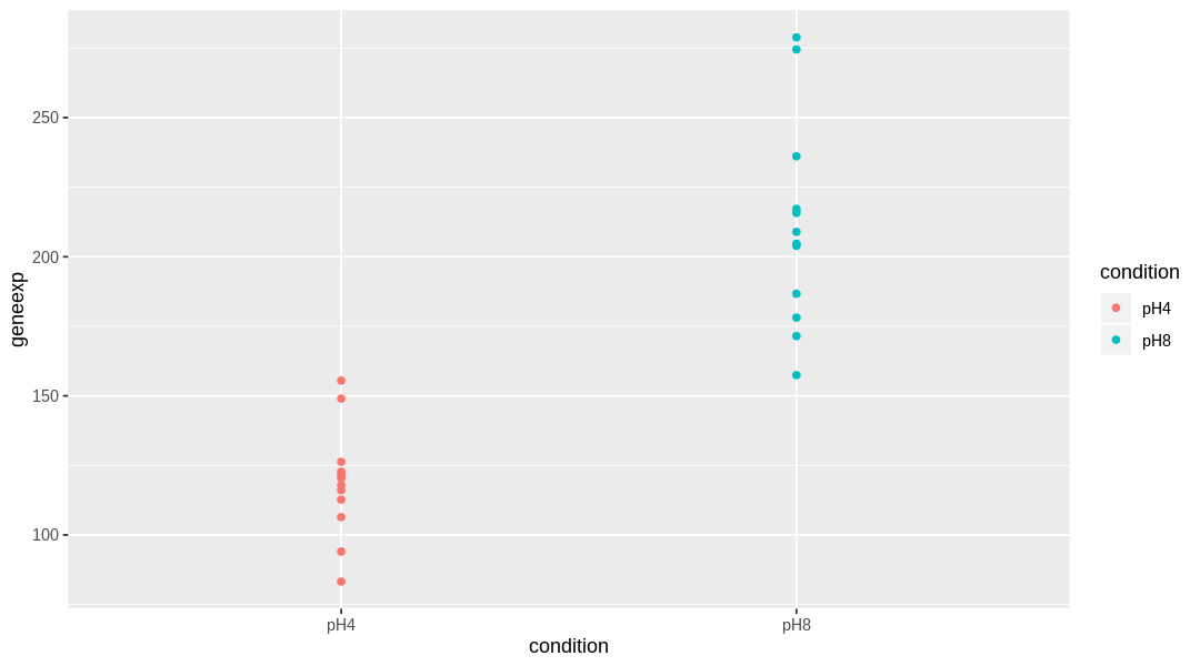
### Add color

myDEplot <- function(mydds, geneid, grpvar, mergelab) {
    mydat <- myDEplotData(mydds, geneid, mergelab)
    ggplot(mydat, aes_string(x=grpvar, y = "geneexp", col = grpvar))+ geom_point()
}
myDEplot(dds2019, "CNAG_00003", "condition", "Label")
[53]:
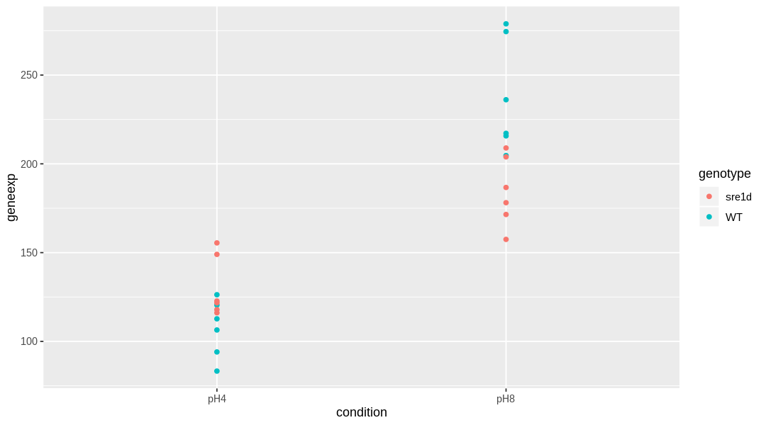
### Alow for coloring with respect to another factor
myDEplot <- function(mydds, geneid, grpvar, colvar, mergelab) {
    mydat <- myDEplotData(mydds, geneid, mergelab)
    ggplot(mydat, aes_string(x=grpvar, y = "geneexp", col = colvar))+ geom_point()
}
myDEplot(dds2019, "CNAG_00003", "condition", "genotype", "Label")
[54]:
sessionInfo()
R version 3.6.0 (2019-04-26)
Platform: x86_64-pc-linux-gnu (64-bit)
Running under: Debian GNU/Linux 9 (stretch)

Matrix products: default
BLAS:   /usr/lib/openblas-base/libblas.so.3
LAPACK: /usr/lib/libopenblasp-r0.2.19.so

locale:
 [1] LC_CTYPE=en_US.UTF-8       LC_NUMERIC=C
 [3] LC_TIME=en_US.UTF-8        LC_COLLATE=en_US.UTF-8
 [5] LC_MONETARY=en_US.UTF-8    LC_MESSAGES=en_US.UTF-8
 [7] LC_PAPER=en_US.UTF-8       LC_NAME=C
 [9] LC_ADDRESS=C               LC_TELEPHONE=C
[11] LC_MEASUREMENT=en_US.UTF-8 LC_IDENTIFICATION=C

attached base packages:
[1] parallel  stats4    stats     graphics  grDevices utils     datasets
[8] methods   base

other attached packages:
 [1] RColorBrewer_1.1-2          dendextend_1.12.0
 [3] DESeq2_1.24.0               SummarizedExperiment_1.14.0
 [5] DelayedArray_0.10.0         BiocParallel_1.18.0
 [7] matrixStats_0.54.0          Biobase_2.44.0
 [9] GenomicRanges_1.36.0        GenomeInfoDb_1.20.0
[11] IRanges_2.18.1              S4Vectors_0.22.0
[13] BiocGenerics_0.30.0         forcats_0.4.0
[15] stringr_1.4.0               dplyr_0.8.1
[17] purrr_0.3.2                 readr_1.3.1
[19] tidyr_0.8.3                 tibble_2.1.2
[21] ggplot2_3.1.1               tidyverse_1.2.1

loaded via a namespace (and not attached):
 [1] colorspace_1.4-1       IRdisplay_0.7.0        htmlTable_1.13.1
 [4] XVector_0.24.0         base64enc_0.1-3        rstudioapi_0.10
 [7] bit64_0.9-7            AnnotationDbi_1.46.0   lubridate_1.7.4
[10] xml2_1.2.0             splines_3.6.0          geneplotter_1.62.0
[13] knitr_1.23             zeallot_0.1.0          IRkernel_1.0.1
[16] Formula_1.2-3          jsonlite_1.6           broom_0.5.2
[19] annotate_1.62.0        cluster_2.0.8          compiler_3.6.0
[22] httr_1.4.0             backports_1.1.4        assertthat_0.2.1
[25] Matrix_1.2-17          lazyeval_0.2.2         cli_1.1.0
[28] acepack_1.4.1          htmltools_0.3.6        tools_3.6.0
[31] gtable_0.3.0           glue_1.3.1             GenomeInfoDbData_1.2.1
[34] Rcpp_1.0.1             cellranger_1.1.0       vctrs_0.1.0
[37] nlme_3.1-139           xfun_0.7               rvest_0.3.4
[40] XML_3.98-1.19          zlibbioc_1.30.0        scales_1.0.0
[43] hms_0.4.2              memoise_1.1.0          gridExtra_2.3
[46] rpart_4.1-15           latticeExtra_0.6-28    stringi_1.4.3
[49] RSQLite_2.1.1          genefilter_1.66.0      checkmate_1.9.3
[52] repr_1.0.1             rlang_0.3.4            pkgconfig_2.0.2
[55] bitops_1.0-6           evaluate_0.14          lattice_0.20-38
[58] labeling_0.3           htmlwidgets_1.3        bit_1.1-14
[61] tidyselect_0.2.5       plyr_1.8.4             magrittr_1.5
[64] R6_2.4.0               generics_0.0.2         Hmisc_4.2-0
[67] pbdZMQ_0.3-3           DBI_1.0.0              pillar_1.4.1
[70] haven_2.1.0            foreign_0.8-71         withr_2.1.2
[73] survival_2.44-1.1      RCurl_1.95-4.12        nnet_7.3-12
[76] modelr_0.1.4           crayon_1.3.4           uuid_0.1-2
[79] viridis_0.5.1          locfit_1.5-9.1         grid_3.6.0
[82] readxl_1.3.1           data.table_1.12.2      blob_1.1.1
[85] digest_0.6.19          xtable_1.8-4           munsell_0.5.0
[88] viridisLite_0.3.0