R Graphics

R Graphics Systems

There are 3 different grpahcis systems widely used in R - base, lattice and ggplot2. We will focus on ggplot2 because it provides the most logical approach to plot constructin using a grammar of graphics.

Base

n <- 100
x <- sort(runif(n))
y <- x^2 + x + 1 + 0.2*rnorm(n)

m <- lm(y ~ I(x^2))

options.orig <- options(repr.plot.width=6, repr.plot.height=4)

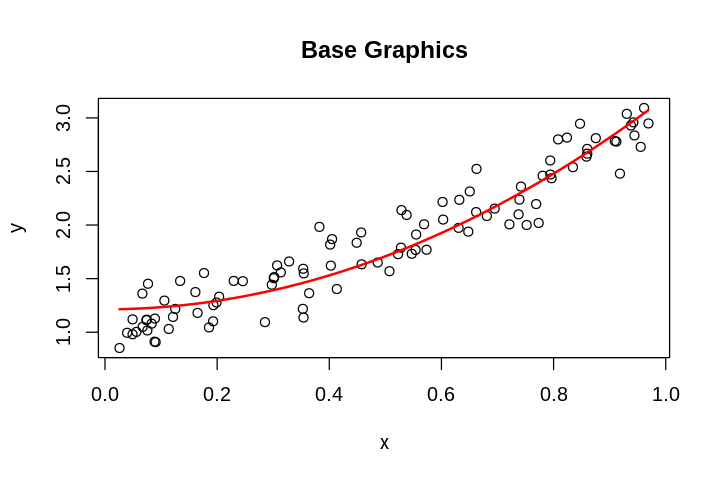
plot(x, y, main="Base Graphics")
lines(x, predict(m), col = "red", lwd = 2)

ggplot2

library(tidyverse)

Registered S3 methods overwritten by 'ggplot2':
  method         from
  [.quosures     rlang
  c.quosures     rlang
  print.quosures rlang
── Attaching packages ─────────────────────────────────────── tidyverse 1.2.1 ──
✔ ggplot2 3.1.1     ✔ purrr   0.3.2
✔ tibble  2.1.2     ✔ dplyr   0.8.1
✔ tidyr   0.8.3     ✔ stringr 1.4.0
✔ readr   1.3.1     ✔ forcats 0.4.0
── Conflicts ────────────────────────────────────────── tidyverse_conflicts() ──
✖ dplyr::filter() masks stats::filter()
✖ dplyr::lag()    masks stats::lag()

ggplto2 only works on data.frame or similar objects

df <- tibble(x=x, y=y)

head(df)

A tibble: 6 × 2

x	y
<dbl>	<dbl>
0.02597720	0.8526721
0.03939677	0.9947642
0.04915126	0.9809143
0.04920200	1.1198401
0.05609914	1.0031721
0.06669788	1.3603442

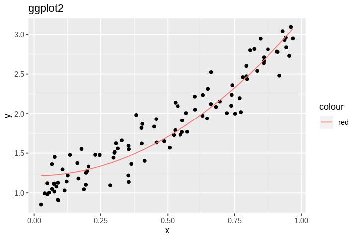
ggplot(df, aes(x=x, y=y)) +
geom_point() +
geom_line(aes(x=x, y=predict(m), color="red")) +
labs(title="ggplot2")

lattice

For more examples, see Getting Started with Lattice Graphics

library(lattice)

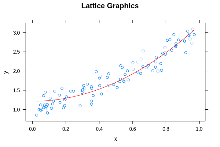
xyplot(y ~ x,
       main = "Lattice Graphics",
       panel = function(x, y, ...) {
             panel.xyplot(x, y, ...)
             panel.lines(x, predict(m), col.line = "red")
         }
       )