Unsupervised Learning¶

Golub data set¶

[1]:

suppressPackageStartupMessages(library(multtest))
suppressPackageStartupMessages(library(golubEsets))
suppressPackageStartupMessages(library(tidyverse))

[2]:

data(Golub_Merge)
dim(Golub_Merge)

Features: 7129
Samples: 72

Extract gene expression values¶

[3]:

golub <- exprs(Golub_Merge)

There are 72 patients and 7192 probe sets.

[4]:

dim(golub)

7129
72

[5]:

head(golub)

A matrix: 6 × 72 of type dbl
	39	40	42	47	48	49	41	43	44	45	⋯	35	36	37	38	28	29	30	31	32	33
AFFX-BioB-5_at	-342	-87	22	-243	-130	-256	-62	86	-146	-187	⋯	7	-213	-25	-72	-4	15	-318	-32	-124	-135
AFFX-BioB-M_at	-200	-248	-153	-218	-177	-249	-23	-36	-74	-187	⋯	-100	-252	-20	-139	-116	-114	-192	-49	-79	-186
AFFX-BioB-3_at	41	262	17	-163	-28	-410	-7	-141	170	312	⋯	-57	136	124	-1	-125	2	-95	49	-37	-70
AFFX-BioC-5_at	328	295	276	182	266	24	142	252	174	142	⋯	132	318	325	392	241	193	312	230	330	337
AFFX-BioC-3_at	-224	-226	-211	-289	-170	-535	-233	-201	-32	114	⋯	-377	-209	-396	-324	-191	-51	-139	-367	-188	-407
AFFX-BioDn-5_at	-427	-493	-250	-268	-326	-810	-284	-384	-318	-148	⋯	-478	-557	-464	-510	-411	-155	-344	-508	-423	-566

For this exercise, we consider the probe values to be variables and the patients to be observations, so it is convenient to work with the matrix transpose.

[6]:

golub <- t(golub)

[7]:

dim(golub)

72
7129

[8]:

golub[1:3, ]

A matrix: 3 × 7129 of type dbl
	AFFX-BioB-5_at	AFFX-BioB-M_at	AFFX-BioB-3_at	AFFX-BioC-5_at	AFFX-BioC-3_at	AFFX-BioDn-5_at	AFFX-BioDn-3_at	AFFX-CreX-5_at	AFFX-CreX-3_at	AFFX-BioB-5_st	⋯	U48730_at	U58516_at	U73738_at	X06956_at	X16699_at	X83863_at	Z17240_at	L49218_f_at	M71243_f_at	Z78285_f_at
39	-342	-200	41	328	-224	-427	-656	-292	137	-144	⋯	277	1023	67	214	-135	1074	475	48	168	-70
40	-87	-248	262	295	-226	-493	367	-452	194	162	⋯	83	529	-295	352	-67	67	263	-33	-33	-21
42	22	-153	17	276	-211	-250	55	-141	0	500	⋯	413	399	16	558	24	893	297	6	1971	-42

Distances¶

Pairwise distance between first 3 patinets¶

[9]:

dist(golub[1:3,])

          39        40
40 101530.75
42  94405.04  89502.29

[10]:

dist(golub[1:3,], diag = TRUE)

          39        40        42
    0.00
101530.75      0.00
94405.04  89502.29      0.00

[11]:

dist(golub[1:3,], diag = TRUE, upper=TRUE)

          39        40        42
    0.00 101530.75  94405.04
101530.75      0.00  89502.29
94405.04  89502.29      0.00

Manual calculation¶

Euclidean distance is just the n-dimensional application of Pythagoras theorem.

If we have points \(x = (0,0)\) and \(y = (3, 4)\), then the distance between \(x\) and \(y\) is

\[\sqrt{(3-0)^2 + (4-0)^2} = 5\]

We write a vectorized calculation of the above.

[12]:

distance <- function(x, y) { sqrt(sum((x - y)^2))}

[13]:

x <- golub[1,]
y <- golub[2,]
round(distance(x, y), 2)

101530.75

Ordination¶

MDS¶

[14]:

mds <- as.data.frame(cmdscale(dist(golub), k = 2))

[15]:

dim(mds)

72
2

[16]:

phenotype <- Golub_Merge@phenoData@data$ALL.AML

[17]:

mds <- mds %>% mutate(phenotype=phenotype)

[18]:

head(mds)

A data.frame: 6 × 3
V1	V2	phenotype
<dbl>	<dbl>	<fct>
23228.24839	-10207.142	ALL
7327.10741	-8114.544	ALL
-5088.36719	-2548.717	ALL
46738.68452	-8792.756	ALL
-39906.71218	-23179.919	ALL
-37.91955	-9771.907	ALL

[19]:

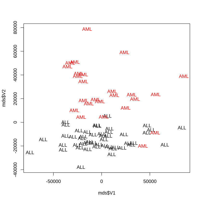
plot(mds$V1, mds$V2, type="n")
text(mds$V1, mds$V2, labels = mds$phenotype, col=as.integer(mds$phenotype))

../_images/cliburn_R05_Unsupervised_Learning_More_Examples_28_0.png

PCA¶

[20]:

pca <- as.data.frame(prcomp(golub, center=TRUE, scale=TRUE, rank=2)$x)

[21]:

dim(pca)

72
2

[22]:

pca <- pca %>% mutate(phenotype=phenotype)

[23]:

head(pca)

A data.frame: 6 × 3
PC1	PC2	phenotype
<dbl>	<dbl>	<fct>
-5.829016	18.985914	ALL
-8.364993	22.877479	ALL
12.928473	-3.996856	ALL
32.254056	-5.525024	ALL
-4.218081	-56.824360	ALL
-65.275849	22.817599	ALL

[24]:

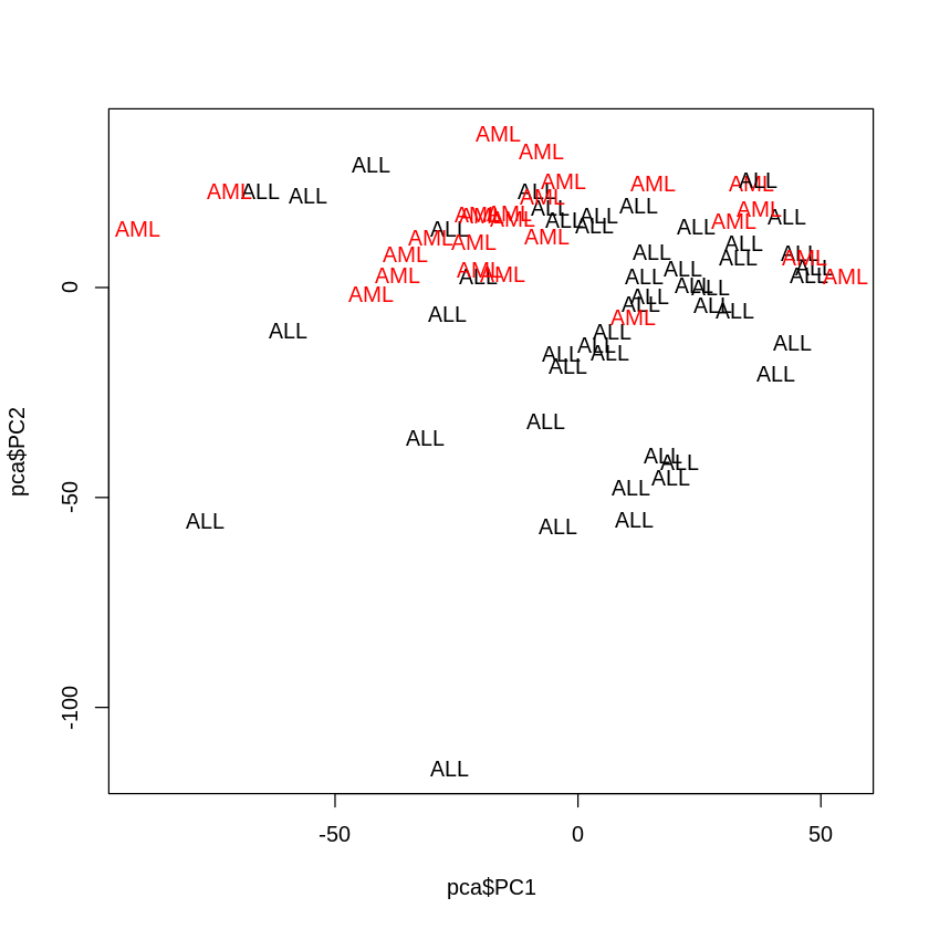
plot(pca$PC1, pca$PC2, type="n")
text(pca$PC1, pca$PC2, labels = pca$phenotype, col=as.integer(pca$phenotype))

../_images/cliburn_R05_Unsupervised_Learning_More_Examples_34_0.png

Preserving the distances¶

Scale to have zero mean and unit standard deviation¶

[25]:

scexpdat <- scale(golub)

[26]:

dim(scexpdat)

72
7129

Check¶

[27]:

apply(scexpdat[, 1:4], 2, mean)

AFFX-BioB-5_at: -7.84141692068388e-17
AFFX-BioB-M_at: -4.46028727069731e-18
AFFX-BioB-3_at: 1.49183207261304e-17
AFFX-BioC-5_at: -5.05117745470191e-17

[28]:

apply(scexpdat[, 1:4], 2, sd)

AFFX-BioB-5_at: 1
AFFX-BioB-M_at: 1
AFFX-BioB-3_at: 1
AFFX-BioC-5_at: 1

Using `dplyr`¶

[29]:

as.data.frame(scexpdat) %>%
select(1:4) %>%
summarise_all(mean) %>%
round

A data.frame: 1 × 4
AFFX-BioB-5_at	AFFX-BioB-M_at	AFFX-BioB-3_at	AFFX-BioC-5_at
<dbl>	<dbl>	<dbl>	<dbl>
0	0	0	0

[30]:

as.data.frame(scexpdat) %>%
select(1:4) %>%
summarise_all(sd) %>%
round

A data.frame: 1 × 4
AFFX-BioB-5_at	AFFX-BioB-M_at	AFFX-BioB-3_at	AFFX-BioC-5_at
<dbl>	<dbl>	<dbl>	<dbl>
1	1	1	1

Clustering¶

Agglomerative hierarchical clustering (AHC)¶

[31]:

names = c("ATL", "BOS", "ORD", "DCA")
airports <- c(0, 934, 585, 542, 934, 0, 853, 392,
              585, 853, 0, 598, 542, 392, 598, 0)
airports <- matrix(airports, ncol=4, byrow=F, dimnames = list(names, names))

[32]:

airports

A matrix: 4 × 4 of type dbl
	ATL	BOS	ORD	DCA
ATL	0	934	585	542
BOS	934	0	853	392
ORD	585	853	0	598
DCA	542	392	598	0

[33]:

as.dist(airports)

    ATL BOS ORD
BOS 934
ORD 585 853
DCA 542 392 598

[34]:

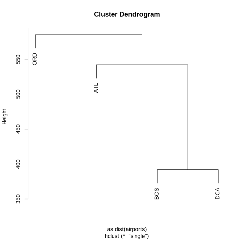
tree <- hclust(as.dist(airports), method="single")
plot(tree)

../_images/cliburn_R05_Unsupervised_Learning_More_Examples_50_0.png

[35]:

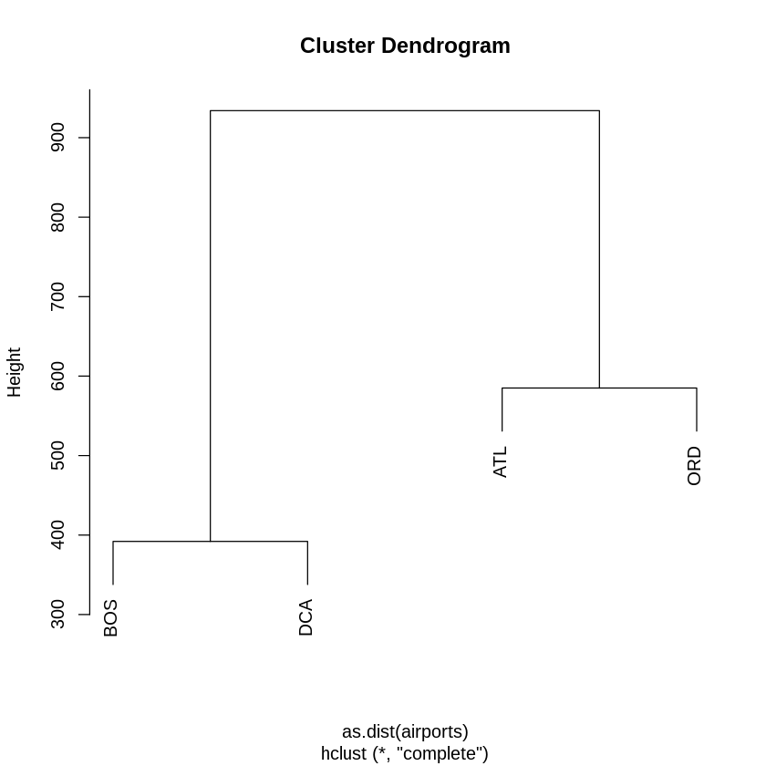
tree <- hclust(as.dist(airports), method="complete")
plot(tree)

../_images/cliburn_R05_Unsupervised_Learning_More_Examples_51_0.png

Road-trip USA¶

[36]:

plot(hclust(UScitiesD, method="complete"))

../_images/cliburn_R05_Unsupervised_Learning_More_Examples_53_0.png

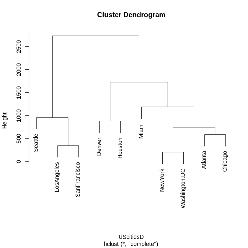
A trip to Europe¶

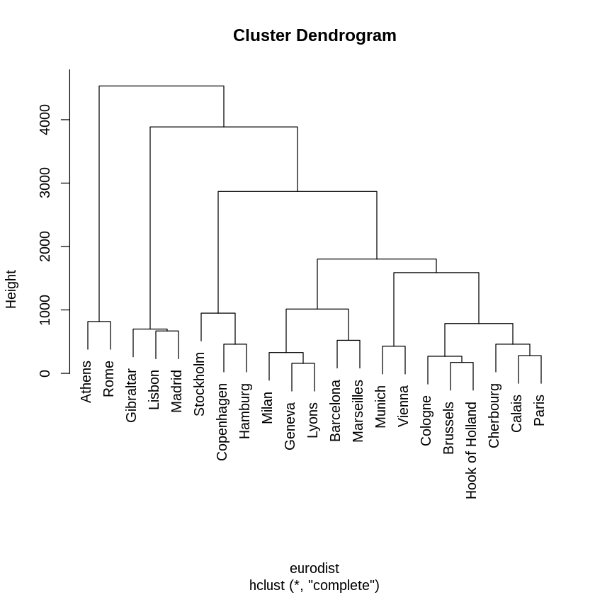
[37]:

plot(hclust(eurodist, method="complete"))

../_images/cliburn_R05_Unsupervised_Learning_More_Examples_55_0.png

[38]:

eurotree <- hclust(eurodist, method="complete")

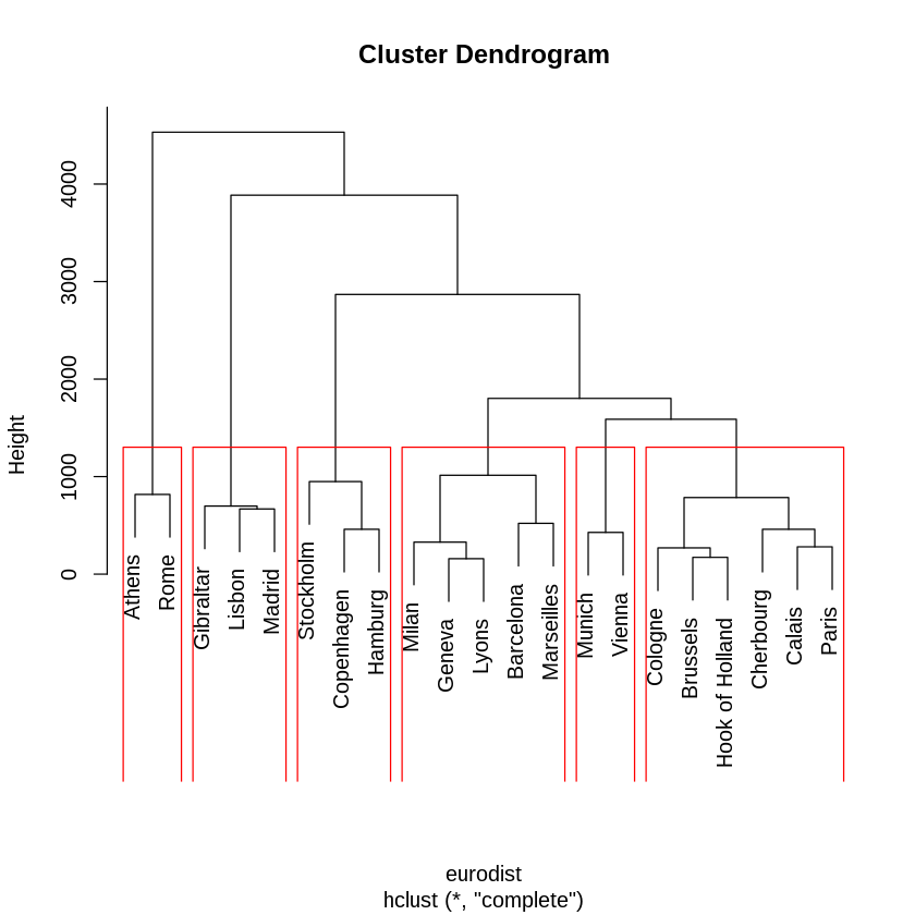
Find clusters by height¶

[39]:

groups <- cutree(tree = eurotree, h = 1500)
data.frame(groups) %>%
rownames_to_column("city") %>%
arrange(groups)

A data.frame: 21 × 2
city	groups
<chr>	<int>
Athens	1
Rome	1
Barcelona	2
Geneva	2
Lyons	2
Marseilles	2
Milan	2
Brussels	3
Calais	3
Cherbourg	3
Cologne	3
Hook of Holland	3
Paris	3
Copenhagen	4
Hamburg	4
Stockholm	4
Gibraltar	5
Lisbon	5
Madrid	5
Munich	6
Vienna	6

[40]:

plot(eurotree)
rect.hclust(eurotree, h=1500, border = "red")

../_images/cliburn_R05_Unsupervised_Learning_More_Examples_59_0.png

Find clusters by number¶

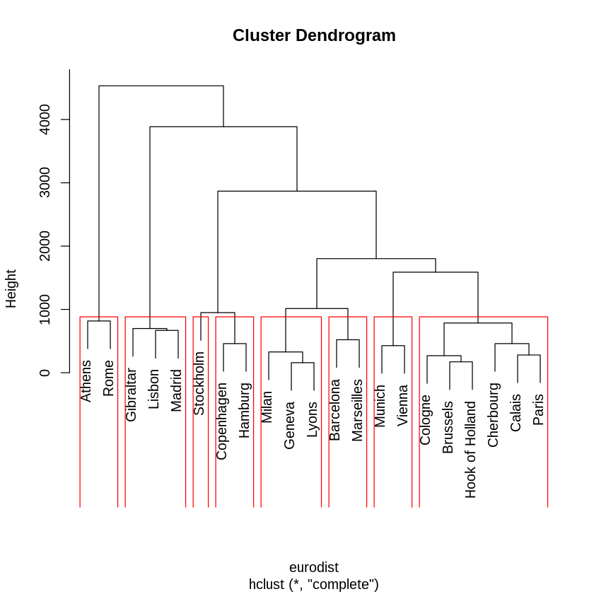
[41]:

groups <- cutree(tree = eurotree, k = 8)
data.frame(groups) %>%
rownames_to_column("city") %>%
arrange(groups)

A data.frame: 21 × 2
city	groups
<chr>	<int>
Athens	1
Rome	1
Barcelona	2
Marseilles	2
Brussels	3
Calais	3
Cherbourg	3
Cologne	3
Hook of Holland	3
Paris	3
Copenhagen	4
Hamburg	4
Geneva	5
Lyons	5
Milan	5
Gibraltar	6
Lisbon	6
Madrid	6
Munich	7
Vienna	7
Stockholm	8

[42]:

plot(eurotree)
rect.hclust(eurotree, k=8, border = "red")

../_images/cliburn_R05_Unsupervised_Learning_More_Examples_62_0.png

k-means clustering¶

[43]:

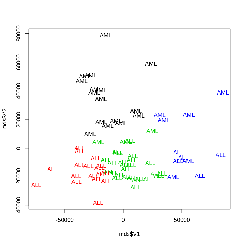
kmeans.golub <- kmeans(golub, centers=4)

[44]:

plot(mds$V1, mds$V2, type="n")
text(mds$V1, mds$V2, labels = mds$phenotype, col=as.integer(kmeans.golub$cluster))

../_images/cliburn_R05_Unsupervised_Learning_More_Examples_65_0.png

Grouped by data source¶

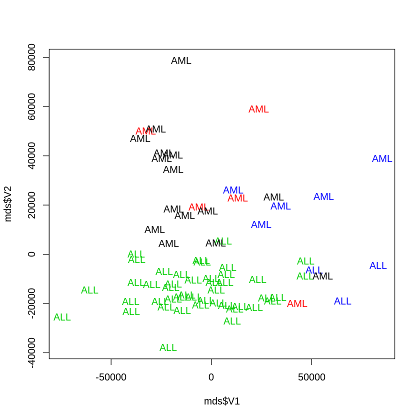
[45]:

plot(mds$V1, mds$V2, type="n")
text(mds$V1, mds$V2, labels = mds$phenotype,
     col=as.integer(Golub_Merge@phenoData@data$Source))

../_images/cliburn_R05_Unsupervised_Learning_More_Examples_67_0.png

Semi-supervised learning (Noise discovery)¶

[46]:

suppressPackageStartupMessages(library(genefilter))
suppressPackageStartupMessages(library(pheatmap))

Simulate noise data set¶

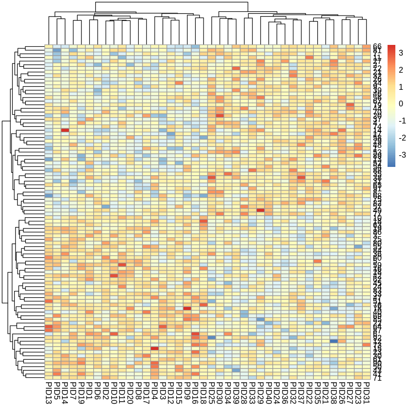
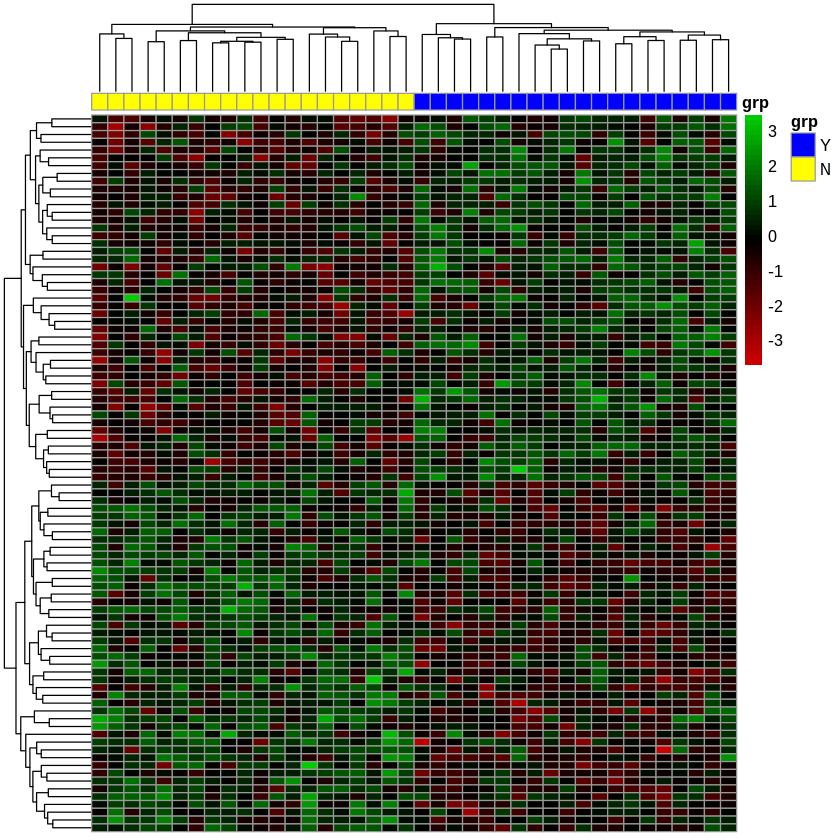
Note that EVERY expression value is drawn from a standard normal distribution. Hence there should not be any meaningful distinction between the “groups”.

[47]:

m <- 20000 # number of genes
n <- 20 # number of subjects
alpha <- 0.005

grp <- factor(rep(c('N', 'Y'), c(n, n)))
genes <- paste("Gene", 1:m, sep="")
subjects <- paste("PID", 1:(2*n), sep="")
expr <- matrix(rnorm(2 * n * m), m, 2 * n)
rownames(expr) <- genes
colnames(expr) <- subjects

Find genes that are different across group at specified significance level¶

[48]:

pvals <- rowttests(expr, grp)$p.value

[49]:

df <- data.frame(expr, pvals)

[50]:

top.genes <- df %>%
filter(pvals < alpha) %>%
select(-pvals)

[51]:

dim(top.genes)

92
40

Show heatmap and AHC clustering for top genes¶

[52]:

annot <- data.frame(grp=grp, row.names=colnames(top.genes))

[53]:

head(annot)

A data.frame: 6 × 1
	grp
	<fct>
PID1	N
PID2	N
PID3	N
PID4	N
PID5	N
PID6	N

Simple version of heatmap¶

[54]:

pheatmap(top.genes)

../_images/cliburn_R05_Unsupervised_Learning_More_Examples_81_0.png

Fancy version of heatmap¶

[55]:

pheatmap(top.genes,
         annotation_col = annot,
         color = colorRampPalette(c("red3", "black", "green3"))(50),
         annotation_colors = list(grp = c(Y = "blue", N = "yellow")),
         show_rownames = FALSE, show_colnames = FALSE,
        )

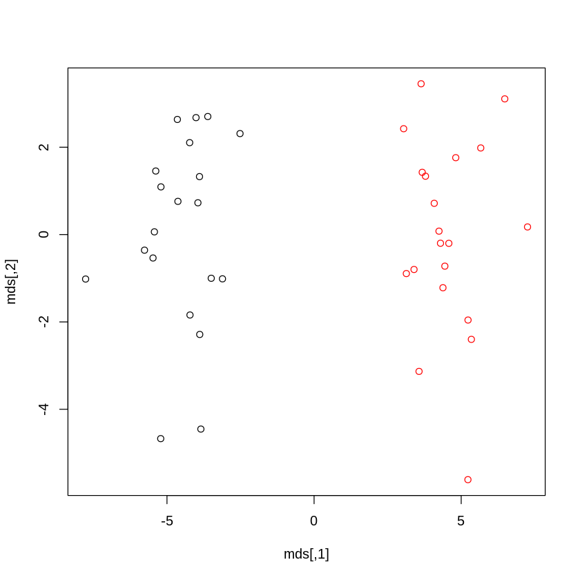
../_images/cliburn_R05_Unsupervised_Learning_More_Examples_83_0.png

MDS of top genes¶

[56]:

mds <- cmdscale(dist(t(top.genes)))
plot(mds, col=as.integer(grp))

../_images/cliburn_R05_Unsupervised_Learning_More_Examples_85_0.png

Exercise 1

Load the iris data set. Each row has 4 features and a Species label.

Reduce the dimensionality of the features to 2 using each of the methods described above (PCA, MDS).
Plot scatter plots for each method, coloring by Species.
Are the Species separate in these dimensionality-reduced plots?

[ ]:

Exercise 2

Load the iris data set. Each row has 4 features and a Species label.

Scale the data to have zero mean and unit standard deviation
Calculate a pairwise distance matrix (explore different distance measures)
Perform hierarchical clustering (explore different linkage measures)
Plot a dendrogram for the hierarchical clustering, showing 3 clusters (see the rect.hclust function)
Create a scatter plot of the first two features colored by the cluster label (see teh cutree function)

[ ]:

Exercise 3

Load the iris data set. Each row has 4 features and a Species label.

Scale the data to have zero mean and unit standard deviation
Perform k-means clustering using 2,3,4 and 10 clusters
Create a scatter plot of the first two features colored by the cluster label for each cluster number
How could you assess how many clusters is appropriate?

[ ]:

Unsupervised Learning¶

Golub data set¶

Extract gene expression values¶

Distances¶

Pairwise distance between first 3 patinets¶

Manual calculation¶

Ordination¶

MDS¶

PCA¶

Preserving the distances¶

Scale to have zero mean and unit standard deviation¶

Check¶

Using dplyr¶

Clustering¶

Agglomerative hierarchical clustering (AHC)¶

Road-trip USA¶

A trip to Europe¶

Find clusters by height¶

Find clusters by number¶

k-means clustering¶

Grouped by data source¶

Semi-supervised learning (Noise discovery)¶

Simulate noise data set¶

Find genes that are different across group at specified significance level¶

Show heatmap and AHC clustering for top genes¶

Simple version of heatmap¶

Fancy version of heatmap¶

MDS of top genes¶

Using `dplyr`¶