Unsupervised Learning
[1]:
library(tidyverse)
Registered S3 methods overwritten by 'ggplot2':
  method         from
  [.quosures     rlang
  c.quosures     rlang
  print.quosures rlang
── Attaching packages ─────────────────────────────────────── tidyverse 1.2.1 ──
✔ ggplot2 3.1.1     ✔ purrr   0.3.2
✔ tibble  2.1.2     ✔ dplyr   0.8.1
✔ tidyr   0.8.3     ✔ stringr 1.4.0
✔ readr   1.3.1     ✔ forcats 0.4.0
── Conflicts ────────────────────────────────────────── tidyverse_conflicts() ──
✖ dplyr::filter() masks stats::filter()
✖ dplyr::lag()    masks stats::lag()
[2]:
head(iris)
| Sepal.Length | Sepal.Width | Petal.Length | Petal.Width | Species |
|---|---|---|---|---|
| <dbl> | <dbl> | <dbl> | <dbl> | <fct> |
| 5.1 | 3.5 | 1.4 | 0.2 | setosa |
| 4.9 | 3.0 | 1.4 | 0.2 | setosa |
| 4.7 | 3.2 | 1.3 | 0.2 | setosa |
| 4.6 | 3.1 | 1.5 | 0.2 | setosa |
| 5.0 | 3.6 | 1.4 | 0.2 | setosa |
| 5.4 | 3.9 | 1.7 | 0.4 | setosa |
Review of tidyverse
1. How many rows and columns are there in the DataFrame?
[ ]:
2. Show just the Species column and any columns with information about Petal.
[ ]:
3. Show a DataFrame with just two columns showing the Length: Width ratio for Sepal and Petal.
[ ]:
4. Count the number of each species where Sepal.Length is less than 6.
[ ]:
5. Summarize the mean and standard deviation for each measurement grouped by Species.
[ ]:
6. Convert iris to “tall” form and assign the resulting DataFrame to iris_t with three columns Species, Measurement and Value.
[ ]:
Calculating distances
Mathematical conditions for a distance function - positivity, symmetry, triangle inequality.
[5]:
small <- iris %>% select(-Species) %>% sample_n(6)
small
| Sepal.Length | Sepal.Width | Petal.Length | Petal.Width |
|---|---|---|---|
| <dbl> | <dbl> | <dbl> | <dbl> |
| 5.9 | 3.2 | 4.8 | 1.8 |
| 5.0 | 3.4 | 1.6 | 0.4 |
| 4.8 | 3.0 | 1.4 | 0.3 |
| 5.5 | 2.5 | 4.0 | 1.3 |
| 7.1 | 3.0 | 5.9 | 2.1 |
| 6.7 | 3.1 | 4.7 | 1.5 |
Euclidean distance
[6]:
iris %>% select(-Species) -> df
x <- df[1,]
y <- df[2,]
sqrt(sum((y-x)^2))
Distance matrix
[7]:
dist(small)
          1         2         3         4         5
2 3.6124784
3 3.8807216 0.5000000
4 1.2409674 2.7622455 2.9154759
5 1.6673332 5.0941143 5.3646994 2.6570661
6 0.8660254 3.7148351 3.9937451 1.5264338 1.4035669
[8]:
dist(small, upper = T, diag=T)
          1         2         3         4         5         6
1 0.0000000 3.6124784 3.8807216 1.2409674 1.6673332 0.8660254
2 3.6124784 0.0000000 0.5000000 2.7622455 5.0941143 3.7148351
3 3.8807216 0.5000000 0.0000000 2.9154759 5.3646994 3.9937451
4 1.2409674 2.7622455 2.9154759 0.0000000 2.6570661 1.5264338
5 1.6673332 5.0941143 5.3646994 2.6570661 0.0000000 1.4035669
6 0.8660254 3.7148351 3.9937451 1.5264338 1.4035669 0.0000000
Scaling before distance
[9]:
dist(scale(small), upper=T, diag=T)
         1        2        3        4        5        6
1 0.000000 2.837472 3.074112 2.498835 1.633162 1.017358
2 2.837472 0.000000 1.357298 3.525992 4.217938 3.080620
3 3.074112 1.357298 0.000000 2.680814 4.270058 3.203481
4 2.498835 3.525992 2.680814 0.000000 2.834187 2.427062
5 1.633162 4.217938 4.270058 2.834187 0.000000 1.179145
6 1.017358 3.080620 3.203481 2.427062 1.179145 0.000000
What is the distance matrix is showing?
[10]:
dist(small, method = "maximum", diag=T, upper=T)
    1   2   3   4   5   6
1 0.0 3.2 3.4 0.8 1.2 0.8
2 3.2 0.0 0.4 2.4 4.3 3.1
3 3.4 0.4 0.0 2.6 4.5 3.3
4 0.8 2.4 2.6 0.0 1.9 1.2
5 1.2 4.3 4.5 1.9 0.0 1.2
6 0.8 3.1 3.3 1.2 1.2 0.0
Agglomerative hierarchical clustering
[11]:
iris %>% select(-Species) -> df
[12]:
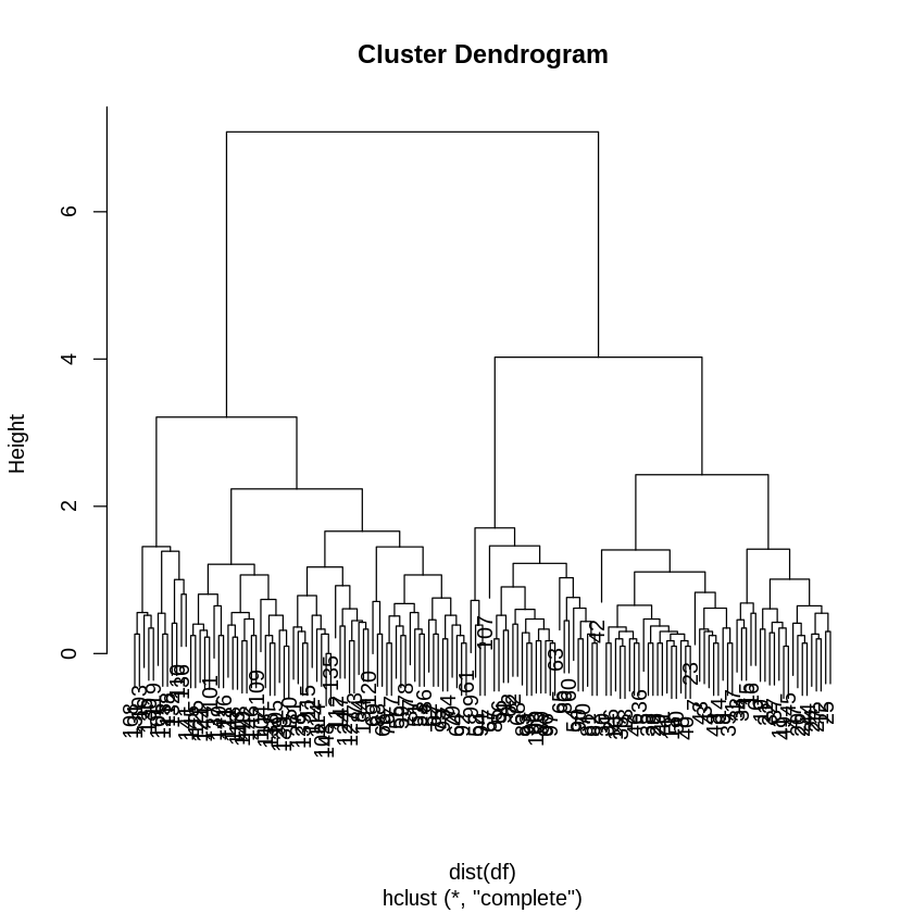
c1 <- hclust(dist(df))
[13]:
plot(c1)
[14]:
z1 <- cutree(c1, 3)
[15]:
z1
- 1
- 1
- 1
- 1
- 1
- 1
- 1
- 1
- 1
- 1
- 1
- 1
- 1
- 1
- 1
- 1
- 1
- 1
- 1
- 1
- 1
- 1
- 1
- 1
- 1
- 1
- 1
- 1
- 1
- 1
- 1
- 1
- 1
- 1
- 1
- 1
- 1
- 1
- 1
- 1
- 1
- 1
- 1
- 1
- 1
- 1
- 1
- 1
- 1
- 1
- 2
- 2
- 2
- 3
- 2
- 3
- 2
- 3
- 2
- 3
- 3
- 3
- 3
- 2
- 3
- 2
- 3
- 3
- 2
- 3
- 2
- 3
- 2
- 2
- 2
- 2
- 2
- 2
- 2
- 3
- 3
- 3
- 3
- 2
- 3
- 2
- 2
- 2
- 3
- 3
- 3
- 2
- 3
- 3
- 3
- 3
- 3
- 2
- 3
- 3
- 2
- 2
- 2
- 2
- 2
- 2
- 3
- 2
- 2
- 2
- 2
- 2
- 2
- 2
- 2
- 2
- 2
- 2
- 2
- 2
- 2
- 2
- 2
- 2
- 2
- 2
- 2
- 2
- 2
- 2
- 2
- 2
- 2
- 2
- 2
- 2
- 2
- 2
- 2
- 2
- 2
- 2
- 2
- 2
- 2
- 2
- 2
- 2
- 2
- 2
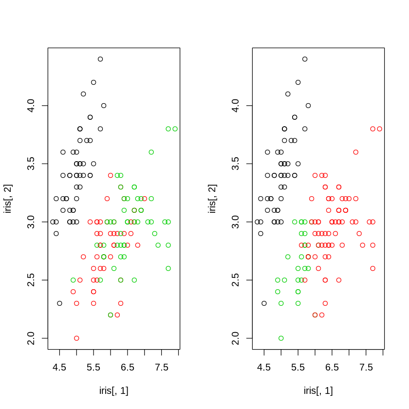
Note that the label values are arbitrary - all we know is that the 1s belong to the same cluster, the 2s belong a another cluster, and the 3s belong to the final cluster. We have no idea what Species thee cluster labels represent, or even if the assignment is “correct” compared to the ground truth.
[16]:
par(mfrow=c(1,2))
plot(iris[, 1], iris[,2], col=iris$Species)
plot(iris[, 1], iris[,2], col=z1)
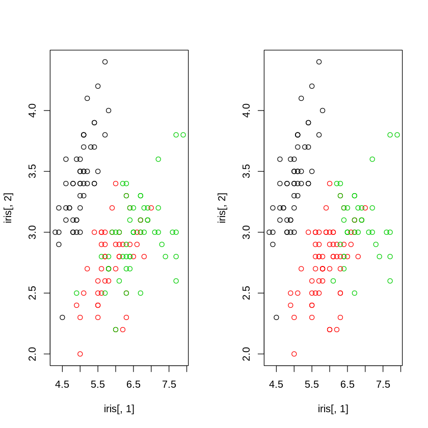
Different linkage methods can give different cluster assignments
[17]:
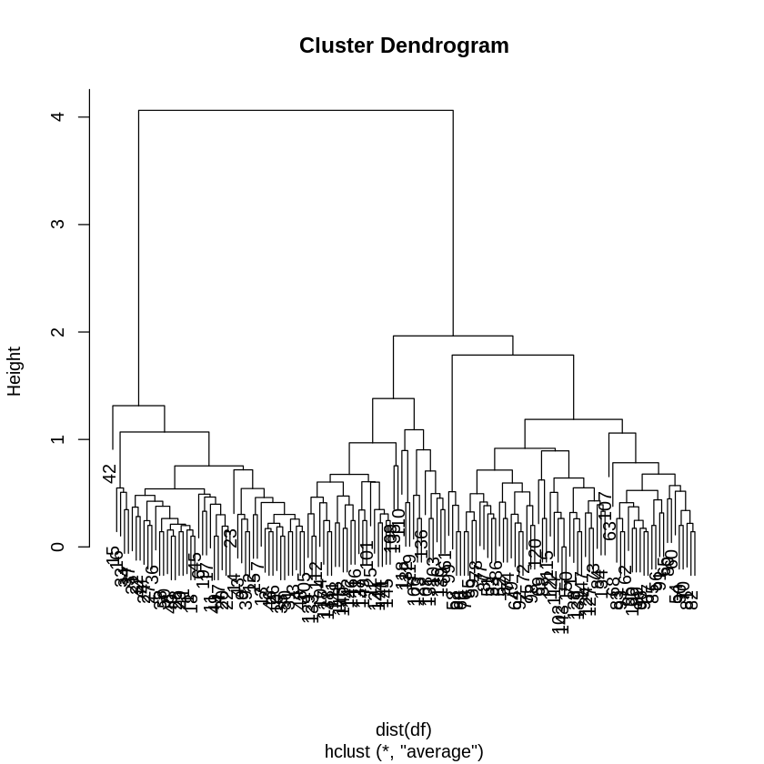
c2 <- hclust(dist(df), method="average")
[18]:
plot(c2)
[19]:
z2 <- cutree(c2, k=3)
[20]:
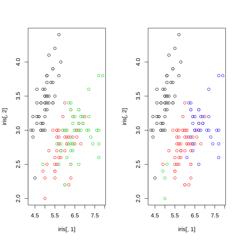
par(mfrow=c(1,2))
plot(iris[, 1], iris[,2], col=iris$Species)
plot(iris[, 1], iris[,2], col=z2)
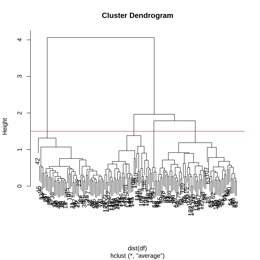
But in reality, we would not know the true number of clusters!
[21]:
plot(c2)
abline(h=1.5, col='red')
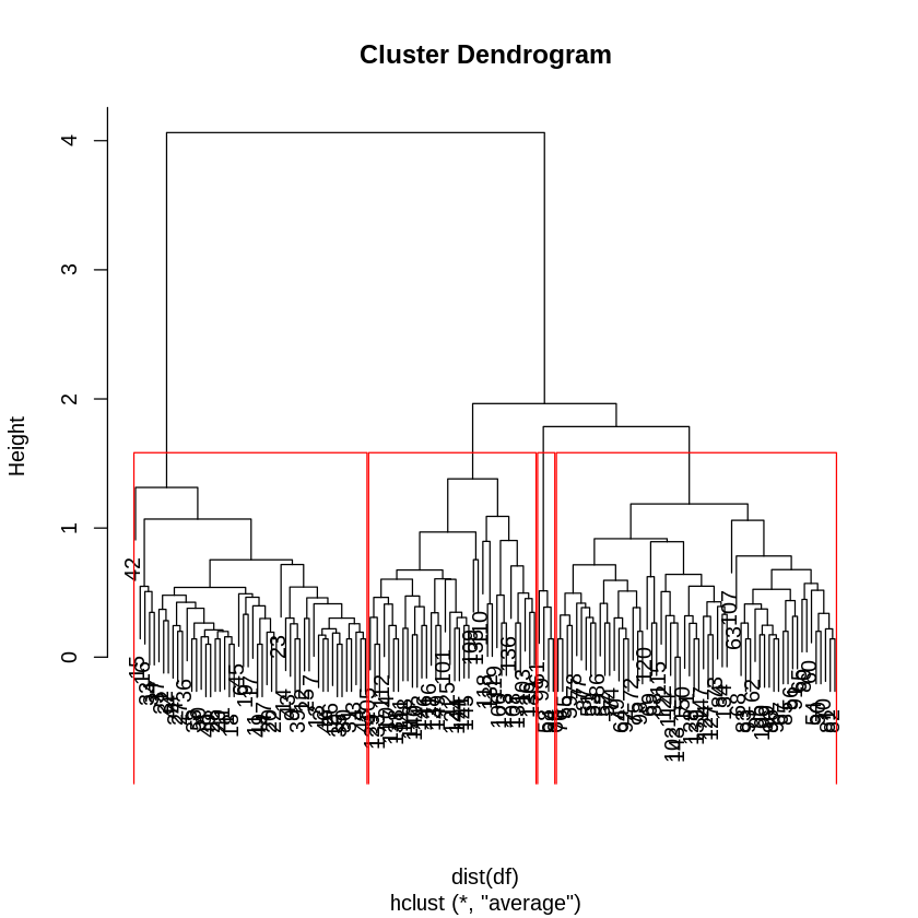
Slightly more informative plot
[22]:
plot(c2)
rect.hclust(c2, h=1.5, border="red")
[23]:
z3 <- cutree(c2, h=1.5)
[24]:
par(mfrow=c(1,2))
plot(iris[, 1], iris[,2], col=iris$Species)
plot(iris[, 1], iris[,2], col=z3)
K-means clustering
[25]:
k1 <- kmeans(dist(df), centers=3)
[26]:
str(k1)
List of 9
 $ cluster     : Named int [1:150] 2 2 2 2 2 2 2 2 2 2 ...
  ..- attr(*, "names")= chr [1:150] "1" "2" "3" "4" ...
 $ centers     : num [1:3, 1:150] 5.095 0.5 3.464 5.146 0.622 ...
  ..- attr(*, "dimnames")=List of 2
  .. ..$ : chr [1:3] "1" "2" "3"
  .. ..$ : chr [1:150] "1" "2" "3" "4" ...
 $ totss       : num 55479
 $ withinss    : num [1:3] 1745 495 2593
 $ tot.withinss: num 4833
 $ betweenss   : num 50646
 $ size        : int [1:3] 38 50 62
 $ iter        : int 2
 $ ifault      : int 0
 - attr(*, "class")= chr "kmeans"
[27]:
as.vector(k1$cluster)
- 2
- 2
- 2
- 2
- 2
- 2
- 2
- 2
- 2
- 2
- 2
- 2
- 2
- 2
- 2
- 2
- 2
- 2
- 2
- 2
- 2
- 2
- 2
- 2
- 2
- 2
- 2
- 2
- 2
- 2
- 2
- 2
- 2
- 2
- 2
- 2
- 2
- 2
- 2
- 2
- 2
- 2
- 2
- 2
- 2
- 2
- 2
- 2
- 2
- 2
- 3
- 3
- 3
- 3
- 3
- 3
- 3
- 3
- 3
- 3
- 3
- 3
- 3
- 3
- 3
- 3
- 3
- 3
- 3
- 3
- 3
- 3
- 3
- 3
- 3
- 3
- 3
- 1
- 3
- 3
- 3
- 3
- 3
- 3
- 3
- 3
- 3
- 3
- 3
- 3
- 3
- 3
- 3
- 3
- 3
- 3
- 3
- 3
- 3
- 3
- 1
- 3
- 1
- 1
- 1
- 1
- 3
- 1
- 1
- 1
- 1
- 1
- 1
- 3
- 1
- 1
- 1
- 1
- 1
- 3
- 1
- 3
- 1
- 3
- 1
- 1
- 3
- 3
- 1
- 1
- 1
- 1
- 1
- 3
- 1
- 1
- 1
- 1
- 3
- 1
- 1
- 1
- 3
- 1
- 1
- 1
- 3
- 1
- 1
- 3
Finding cluster means
Base R
These incantations are hard to remember. I suggest you stick to tidyverse methods.
[28]:
aggregate(df,by=list(k1$cluster),FUN=mean)
| Group.1 | Sepal.Length | Sepal.Width | Petal.Length | Petal.Width |
|---|---|---|---|---|
| <int> | <dbl> | <dbl> | <dbl> | <dbl> |
| 1 | 6.821053 | 3.065789 | 5.747368 | 2.094737 |
| 2 | 5.006000 | 3.428000 | 1.462000 | 0.246000 |
| 3 | 5.919355 | 2.753226 | 4.390323 | 1.419355 |
dplyr
[29]:
df %>%
mutate(z = k1$cluster)  %>%
group_by(z) %>%
summarise_all(mean) -> centroids
[30]:
centroids
| z | Sepal.Length | Sepal.Width | Petal.Length | Petal.Width |
|---|---|---|---|---|
| <int> | <dbl> | <dbl> | <dbl> | <dbl> |
| 1 | 6.821053 | 3.065789 | 5.747368 | 2.094737 |
| 2 | 5.006000 | 3.428000 | 1.462000 | 0.246000 |
| 3 | 5.919355 | 2.753226 | 4.390323 | 1.419355 |
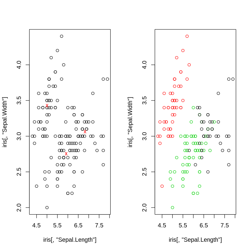
[31]:
par(mfrow=c(1,2))
plot(iris[,"Sepal.Length"], iris[,"Sepal.Width"])
points(centroids[["Sepal.Length"]], centroids[["Sepal.Width"]], col="red",  pch="x")
plot(iris[,"Sepal.Length"], iris[,"Sepal.Width"], col=k1$cluster)
Dimension reduction and ordination
PCA
[32]:
pc <- prcomp(df, center=T, scale=T)
[33]:
str(pc)
List of 5
 $ sdev    : num [1:4] 1.708 0.956 0.383 0.144
 $ rotation: num [1:4, 1:4] 0.521 -0.269 0.58 0.565 -0.377 ...
  ..- attr(*, "dimnames")=List of 2
  .. ..$ : chr [1:4] "Sepal.Length" "Sepal.Width" "Petal.Length" "Petal.Width"
  .. ..$ : chr [1:4] "PC1" "PC2" "PC3" "PC4"
 $ center  : Named num [1:4] 5.84 3.06 3.76 1.2
  ..- attr(*, "names")= chr [1:4] "Sepal.Length" "Sepal.Width" "Petal.Length" "Petal.Width"
 $ scale   : Named num [1:4] 0.828 0.436 1.765 0.762
  ..- attr(*, "names")= chr [1:4] "Sepal.Length" "Sepal.Width" "Petal.Length" "Petal.Width"
 $ x       : num [1:150, 1:4] -2.26 -2.07 -2.36 -2.29 -2.38 ...
  ..- attr(*, "dimnames")=List of 2
  .. ..$ : NULL
  .. ..$ : chr [1:4] "PC1" "PC2" "PC3" "PC4"
 - attr(*, "class")= chr "prcomp"
[34]:
summary(pc)
Importance of components:
                          PC1    PC2     PC3     PC4
Standard deviation     1.7084 0.9560 0.38309 0.14393
Proportion of Variance 0.7296 0.2285 0.03669 0.00518
Cumulative Proportion  0.7296 0.9581 0.99482 1.00000
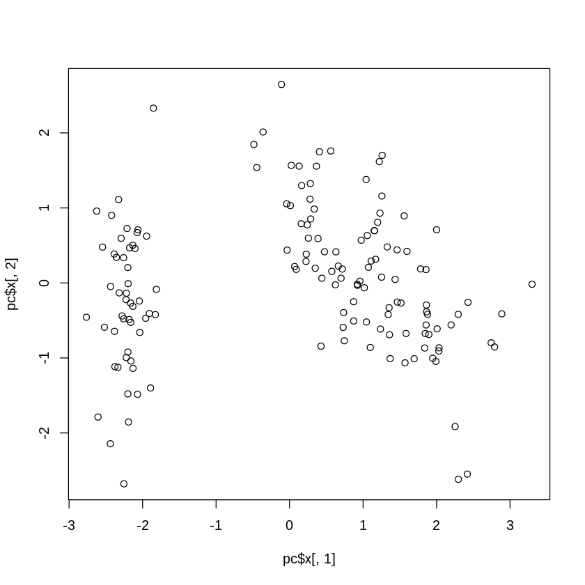
[35]:
plot(pc$x[,1], pc$x[,2])
Classical MDS
[36]:
mds <- cmdscale(dist(df), k = 2)
[37]:
str(mds)
 num [1:150, 1:2] -2.68 -2.71 -2.89 -2.75 -2.73 ...
 - attr(*, "dimnames")=List of 2
  ..$ : NULL
  ..$ : NULL
[38]:
summary(mds)
      V1                V2
Min.   :-3.2238   Min.   :-1.26597
1st Qu.:-2.5303   1st Qu.:-0.32542
Median : 0.5546   Median :-0.02216
Mean   : 0.0000   Mean   : 0.00000
3rd Qu.: 1.5501   3rd Qu.: 0.32492
Max.   : 3.7956   Max.   : 1.37417
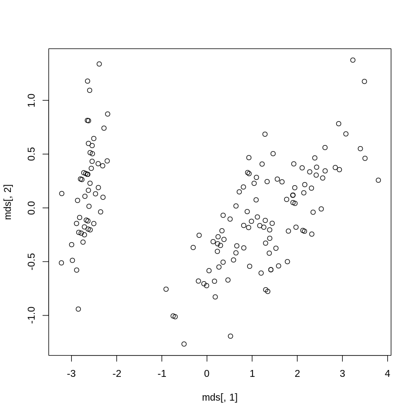
[39]:
plot(mds[,1], mds[,2])
Heatmaps
[40]:
library(pheatmap)
[41]:
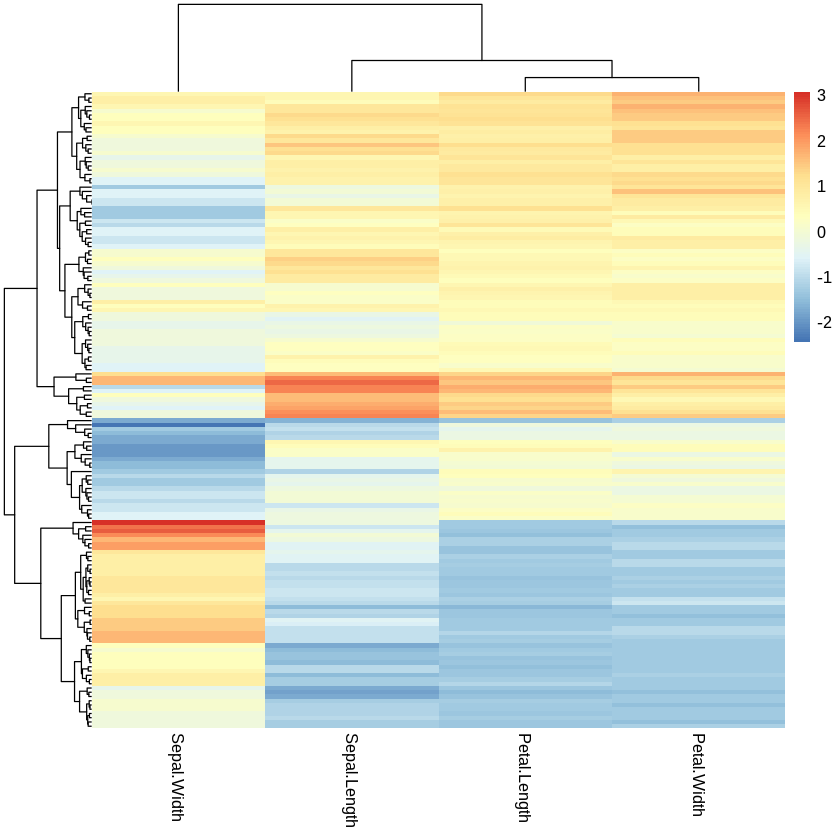
pheatmap(scale(df))
[42]:
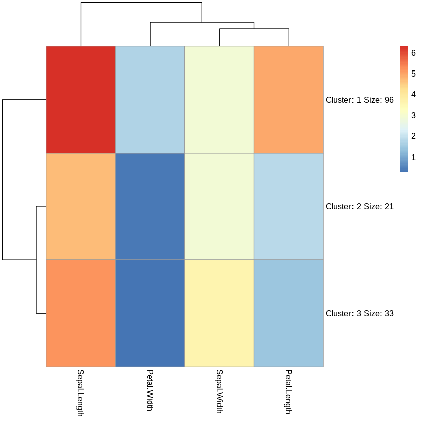
pheatmap(df, kmeans_k = 3)
[43]:
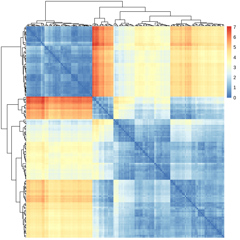
pheatmap(dist(df))
[ ]: